

Abyssal Mixing in the Laboratory
233
Ω
θ [rad]
π
π
π
π
0.1
0.2
0.3
0.4
0.5
0.6
0.7
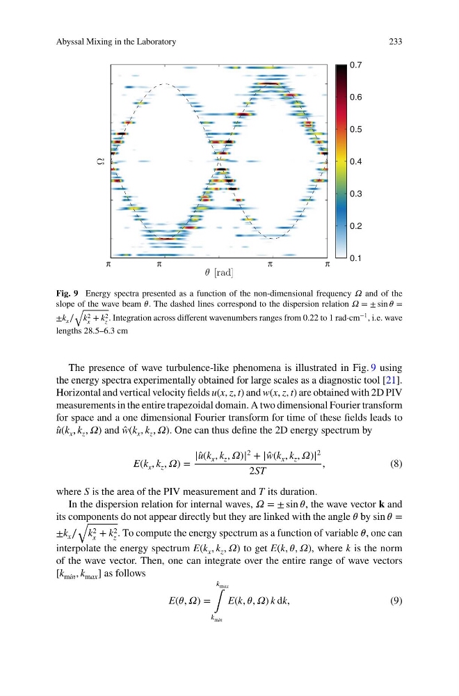
Fig. 9 Energy spectra presented as a function of the non-dimensional frequency í µí»º and of the
slope of the wave beam í µí¼. The dashed lines correspond to the dispersion relation í µí»º = ± sin í µí¼ =
±k x ∕
√
k 2
x
+ k 2
z
. Integration across different wavenumbers ranges from 0.22 to 1 rad⋅cm −1 , i.e. wave
lengths 28.5–6.3 cm
The presence of wave turbulence-like phenomena is illustrated in Fig. 9 using
the energy spectra experimentally obtained for large scales as a diagnostic tool [21].
Horizontal and vertical velocity fields u(x, z, t) and w(x, z, t) are obtained with 2D PIV
measurements in the entire trapezoidal domain. A two dimensional Fourier transform
for space and a one dimensional Fourier transform for time of these fields leads to
̂
u(k x , k z , í µí»º) and ̂
w(k x , k z , í µí»º). One can thus define the 2D energy spectrum by
E(k x , k z , í µí»º) =
|̂ u(k x , k z , í µí»º)|
2 + | ̂
w(k x , k z , í µí»º)|
2
2ST
,
(8)
where S is the area of the PIV measurement and T its duration.
In the dispersion relation for internal waves, í µí»º = ± sin í µí¼, the wave vector í µí°¤ and
its components do not appear directly but they are linked with the angle í µí¼ by sin í µí¼ =
±k x ∕
√
k 2
x
+ k 2
z
. To compute the energy spectrum as a function of variable í µí¼, one can
interpolate the energy spectrum E(k x , k z , í µí»º) to get E(k, í µí¼, í µí»º), where k is the norm
of the wave vector. Then, one can integrate over the entire range of wave vectors
[k min , k max ] as follows
E(í µí¼, í µí»º) =
k max
∫
k min
E(k, í µí¼, í µí»º) k dk,
(9)
233
Ω
θ [rad]
π
π
π
π
0.1
0.2
0.3
0.4
0.5
0.6
0.7
Fig. 9 Energy spectra presented as a function of the non-dimensional frequency í µí»º and of the
slope of the wave beam í µí¼. The dashed lines correspond to the dispersion relation í µí»º = ± sin í µí¼ =
±k x ∕
√
k 2
x
+ k 2
z
. Integration across different wavenumbers ranges from 0.22 to 1 rad⋅cm −1 , i.e. wave
lengths 28.5–6.3 cm
The presence of wave turbulence-like phenomena is illustrated in Fig. 9 using
the energy spectra experimentally obtained for large scales as a diagnostic tool [21].
Horizontal and vertical velocity fields u(x, z, t) and w(x, z, t) are obtained with 2D PIV
measurements in the entire trapezoidal domain. A two dimensional Fourier transform
for space and a one dimensional Fourier transform for time of these fields leads to
̂
u(k x , k z , í µí»º) and ̂
w(k x , k z , í µí»º). One can thus define the 2D energy spectrum by
E(k x , k z , í µí»º) =
|̂ u(k x , k z , í µí»º)|
2 + | ̂
w(k x , k z , í µí»º)|
2
2ST
,
(8)
where S is the area of the PIV measurement and T its duration.
In the dispersion relation for internal waves, í µí»º = ± sin í µí¼, the wave vector í µí°¤ and
its components do not appear directly but they are linked with the angle í µí¼ by sin í µí¼ =
±k x ∕
√
k 2
x
+ k 2
z
. To compute the energy spectrum as a function of variable í µí¼, one can
interpolate the energy spectrum E(k x , k z , í µí»º) to get E(k, í µí¼, í µí»º), where k is the norm
of the wave vector. Then, one can integrate over the entire range of wave vectors
[k min , k max ] as follows
E(í µí¼, í µí»º) =
k max
∫
k min
E(k, í µí¼, í µí»º) k dk,
(9)