

∂
2 p
∂z 2 −
1
c 2
∂
2 p
∂y 2 +
∂
2 p
∂x 2
= − iω Qρ 0 δðx − x 0 Þδðy − y 0 Þδðz − z 0 Þ ̸ c
2 ,
ð2:4Þ
∂p
∂z
= 0 at z = 0,
∂p
∂z
−
γ
c 2
∂p
∂y
= 0 at z = − γ y.
ð2:5Þ
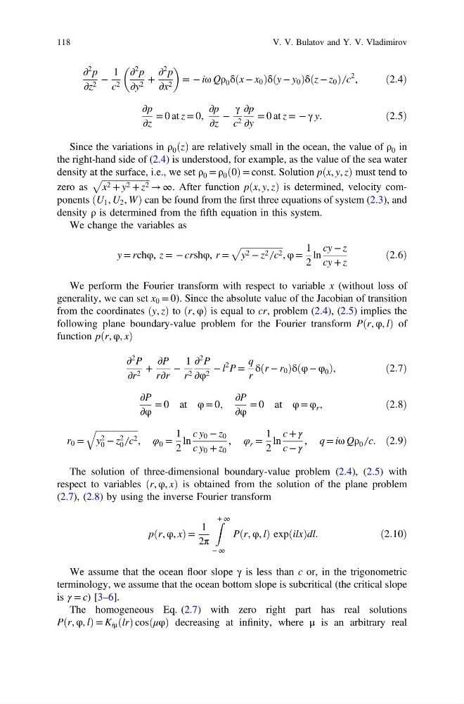
Since the variations in ρ 0 ðzÞ are relatively small in the ocean, the value of ρ 0 in
the right-hand side of (2.4) is understood, for example, as the value of the sea water
density at the surface, i.e., we set ρ 0 = ρ 0 ð0Þ = const. Solution pðx, y, zÞ must tend to
zero as
ffiffiffiffiffiffiffiffiffiffiffiffiffiffiffiffiffiffiffiffiffiffi
x 2 + y 2 + z 2
p
→ ∞. After function pðx, y, zÞ is determined, velocity components ðU 1 , U 2 , WÞ can be found from the first three equations of system (2.3), and
density ρ is determined from the fifth equation in this system.
We change the variables as
y = rchφ, z = − crshφ, r =
ffiffiffiffiffiffiffiffiffiffiffiffiffiffiffiffiffiffiffi
y 2 − z 2 ̸ c 2
p
, φ =
1
2
ln
cy − z
cy + z
ð2:6Þ
We perform the Fourier transform with respect to variable x (without loss of
generality, we can set x 0 = 0). Since the absolute value of the Jacobian of transition
from the coordinates ðy, zÞ to ðr, φÞ is equal to cr, problem (2.4), (2.5) implies the
following plane boundary-value problem for the Fourier transform Pðr, φ, lÞ of
function pðr, φ, xÞ
∂
2 P
∂r 2 +
∂P
r∂r
−
1
r 2
∂
2 P
∂φ 2 − l
2 P =
q
r
δðr − r 0 Þδðφ − φ 0 Þ,
ð2:7Þ
∂P
∂φ
= 0 at φ = 0;
∂P
∂φ
= 0 at φ = φ r ,
ð2:8Þ
r 0 =
ffiffiffiffiffiffiffiffiffiffiffiffiffiffiffiffiffiffiffi
y 2
0 − z 2
0 ̸ c 2
q
, φ 0 =
1
2
ln
c y 0 − z 0
c y 0 + z 0
, φ r =
1
2
ln
c + γ
c − γ
, q = iω Qρ 0 ̸ c. ð2:9Þ
The solution of three-dimensional boundary-value problem (2.4), (2.5) with
respect to variables ðr, φ, xÞ is obtained from the solution of the plane problem
(2.7), (2.8) by using the inverse Fourier transform
pðr, φ, xÞ =
1
2π
Z + ∞
− ∞
Pðr, φ, lÞ expðilxÞdl.
ð2:10Þ
We assume that the ocean floor slope γ is less than c or, in the trigonometric
terminology, we assume that the ocean bottom slope is subcritical (the critical slope
is γ = c) [3–6].
The homogeneous Eq. (2.7) with zero right part has real solutions
Pðr, φ, lÞ = K iμ ðlrÞ cosðμφÞ decreasing at infinity, where μ is an arbitrary real
118
V. V. Bulatov and Y. V. Vladimirov
2 p
∂z 2 −
1
c 2
∂
2 p
∂y 2 +
∂
2 p
∂x 2
= − iω Qρ 0 δðx − x 0 Þδðy − y 0 Þδðz − z 0 Þ ̸ c
2 ,
ð2:4Þ
∂p
∂z
= 0 at z = 0,
∂p
∂z
−
γ
c 2
∂p
∂y
= 0 at z = − γ y.
ð2:5Þ
Since the variations in ρ 0 ðzÞ are relatively small in the ocean, the value of ρ 0 in
the right-hand side of (2.4) is understood, for example, as the value of the sea water
density at the surface, i.e., we set ρ 0 = ρ 0 ð0Þ = const. Solution pðx, y, zÞ must tend to
zero as
ffiffiffiffiffiffiffiffiffiffiffiffiffiffiffiffiffiffiffiffiffiffi
x 2 + y 2 + z 2
p
→ ∞. After function pðx, y, zÞ is determined, velocity components ðU 1 , U 2 , WÞ can be found from the first three equations of system (2.3), and
density ρ is determined from the fifth equation in this system.
We change the variables as
y = rchφ, z = − crshφ, r =
ffiffiffiffiffiffiffiffiffiffiffiffiffiffiffiffiffiffiffi
y 2 − z 2 ̸ c 2
p
, φ =
1
2
ln
cy − z
cy + z
ð2:6Þ
We perform the Fourier transform with respect to variable x (without loss of
generality, we can set x 0 = 0). Since the absolute value of the Jacobian of transition
from the coordinates ðy, zÞ to ðr, φÞ is equal to cr, problem (2.4), (2.5) implies the
following plane boundary-value problem for the Fourier transform Pðr, φ, lÞ of
function pðr, φ, xÞ
∂
2 P
∂r 2 +
∂P
r∂r
−
1
r 2
∂
2 P
∂φ 2 − l
2 P =
q
r
δðr − r 0 Þδðφ − φ 0 Þ,
ð2:7Þ
∂P
∂φ
= 0 at φ = 0;
∂P
∂φ
= 0 at φ = φ r ,
ð2:8Þ
r 0 =
ffiffiffiffiffiffiffiffiffiffiffiffiffiffiffiffiffiffiffi
y 2
0 − z 2
0 ̸ c 2
q
, φ 0 =
1
2
ln
c y 0 − z 0
c y 0 + z 0
, φ r =
1
2
ln
c + γ
c − γ
, q = iω Qρ 0 ̸ c. ð2:9Þ
The solution of three-dimensional boundary-value problem (2.4), (2.5) with
respect to variables ðr, φ, xÞ is obtained from the solution of the plane problem
(2.7), (2.8) by using the inverse Fourier transform
pðr, φ, xÞ =
1
2π
Z + ∞
− ∞
Pðr, φ, lÞ expðilxÞdl.
ð2:10Þ
We assume that the ocean floor slope γ is less than c or, in the trigonometric
terminology, we assume that the ocean bottom slope is subcritical (the critical slope
is γ = c) [3–6].
The homogeneous Eq. (2.7) with zero right part has real solutions
Pðr, φ, lÞ = K iμ ðlrÞ cosðμφÞ decreasing at infinity, where μ is an arbitrary real
118
V. V. Bulatov and Y. V. Vladimirov