

Chapter 5. SPATIALLY-COHERENT STRUCTURES
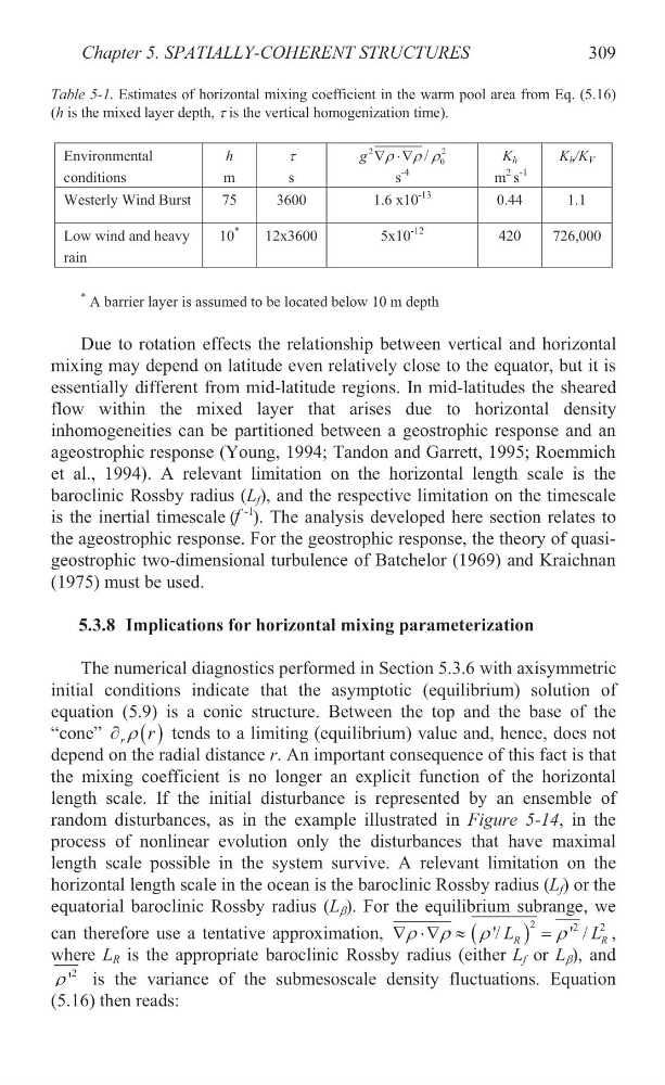
Table 5-1. Estimates of horizontal mixing coefficient in the warm pool area from Eq. (5.16)
(h is the mixed layer depth, Wis the vertical homogenization time).
Environmental
conditions
h
m
W
s
2
2
0
/
g U U U
s
-4
K h
m
2 s
-1
K h /K V
Westerly Wind Burst
75
3600
1.6 x10
-13
0.44
1.1
Low wind and heavy
rain
10
*
12x3600
5x10
-12
420
726,000
* A barrier layer is assumed to be located below 10 m depth
Due to rotation effects the relationship between vertical and horizontal
mixing may depend on latitude even relatively close to the equator, but it is
essentially different from mid-latitude regions. In mid-latitudes the sheared
flow within the mixed layer that arises due to horizontal density
inhomogeneities can be partitioned between a geostrophic response and an
ageostrophic response (Young, 1994; Tandon and Garrett, 1995; Roemmich
et al., 1994). A relevant limitation on the horizontal length scale is the
baroclinic Rossby radius (L f ), and the respective limitation on the timescale
is the inertial timescale (f ). The analysis developed here section relates to
the ageostrophic response. For the geostrophic response, the theory of quasigeostrophic two-dimensional turbulence of Batchelor (1969) and Kraichnan
(1975) must be used.
5.3.8 Implications for horizontal mixing parameterization
The numerical diagnostics performed in Section 5.3.6 with axisymmetric
initial conditions indicate that the asymptotic (equilibrium) solution of
equation (5.9) is a conic structure. Between the top and the base of the
“cone”
r
r
U
w
tends to a limiting (equilibrium) value and, hence, does not
depend on the radial distance r. An important consequence of this fact is that
the mixing coefficient is no longer an explicit function of the horizontal
length scale. If the initial disturbance is represented by an ensemble of
random disturbances, as in the example illustrated in Figure 5-14, in the
process of nonlinear evolution only the disturbances that have maximal
length scale possible in the system survive. A relevant limitation on the
horizontal length scale in the ocean is the baroclinic Rossby radius (L f ) or the
equatorial baroclinic Rossby radius (L E ). For the equilibrium subrange, we
can therefore use a tentative approximation, U U
|
2
2
2
'/
' /
R
R
L
L
U
U
,
where L R is the appropriate baroclinic Rossby radius (either L f or L E ), and
2
'
U is the variance of the submesoscale density fluctuations. Equation
(5.16) then reads:
309
-1
Table 5-1. Estimates of horizontal mixing coefficient in the warm pool area from Eq. (5.16)
(h is the mixed layer depth, Wis the vertical homogenization time).
Environmental
conditions
h
m
W
s
2
2
0
/
g U U U
s
-4
K h
m
2 s
-1
K h /K V
Westerly Wind Burst
75
3600
1.6 x10
-13
0.44
1.1
Low wind and heavy
rain
10
*
12x3600
5x10
-12
420
726,000
* A barrier layer is assumed to be located below 10 m depth
Due to rotation effects the relationship between vertical and horizontal
mixing may depend on latitude even relatively close to the equator, but it is
essentially different from mid-latitude regions. In mid-latitudes the sheared
flow within the mixed layer that arises due to horizontal density
inhomogeneities can be partitioned between a geostrophic response and an
ageostrophic response (Young, 1994; Tandon and Garrett, 1995; Roemmich
et al., 1994). A relevant limitation on the horizontal length scale is the
baroclinic Rossby radius (L f ), and the respective limitation on the timescale
is the inertial timescale (f ). The analysis developed here section relates to
the ageostrophic response. For the geostrophic response, the theory of quasigeostrophic two-dimensional turbulence of Batchelor (1969) and Kraichnan
(1975) must be used.
5.3.8 Implications for horizontal mixing parameterization
The numerical diagnostics performed in Section 5.3.6 with axisymmetric
initial conditions indicate that the asymptotic (equilibrium) solution of
equation (5.9) is a conic structure. Between the top and the base of the
“cone”
r
r
U
w
tends to a limiting (equilibrium) value and, hence, does not
depend on the radial distance r. An important consequence of this fact is that
the mixing coefficient is no longer an explicit function of the horizontal
length scale. If the initial disturbance is represented by an ensemble of
random disturbances, as in the example illustrated in Figure 5-14, in the
process of nonlinear evolution only the disturbances that have maximal
length scale possible in the system survive. A relevant limitation on the
horizontal length scale in the ocean is the baroclinic Rossby radius (L f ) or the
equatorial baroclinic Rossby radius (L E ). For the equilibrium subrange, we
can therefore use a tentative approximation, U U
|
2
2
2
'/
' /
R
R
L
L
U
U
,
where L R is the appropriate baroclinic Rossby radius (either L f or L E ), and
2
'
U is the variance of the submesoscale density fluctuations. Equation
(5.16) then reads:
309
-1