

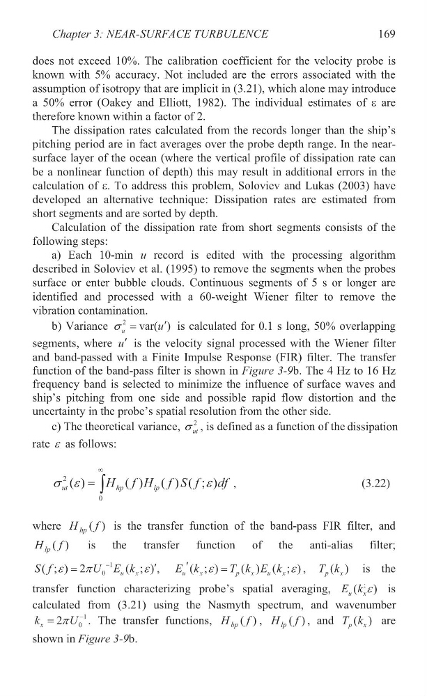
does not exceed 10%. The calibration coefficient for the velocity probe is
known with 5% accuracy. Not included are the errors associated with the
assumption of isotropy that are implicit in (3.21), which alone may introduce
a 50% error (Oakey and Elliott, 1982). The individual estimates of H are
therefore known within a factor of 2.
The dissipation rates calculated from the records longer than the ship’s
pitching period are in fact averages over the probe depth range. In the nearsurface layer of the ocean (where the vertical profile of dissipation rate can
be a nonlinear function of depth) this may result in additional errors in the
calculation of H. To address this problem, Soloviev and Lukas (2003) have
developed an alternative technique: Dissipation rates are estimated from
short segments and are sorted by depth.
Calculation of the dissipation rate from short segments consists of the
following steps:
a) Each 10-min u record is edited with the processing algorithm
described in Soloviev et al. (1995) to remove the segments when the probes
surface or enter bubble clouds. Continuous segments of 5 s or longer are
identified and processed with a 60-weight Wiener filter to remove the
vibration contamination.
b) Variance
2
var( )
u
u
V
c is calculated for 0.1 s long, 50% overlapping
segments, where uc is the velocity signal processed with the Wiener filter
and band-passed with a Finite Impulse Response (FIR) filter. The transfer
function of the band-pass filter is shown in Figure 3-9b. The 4 Hz to 16 Hz
frequency band is selected to minimize the influence of surface waves and
ship’s pitching from one side and possible rapid flow distortion and the
uncertainty in the probe’s spatial resolution from the other side.
c) The theoretical variance,
2
ut
V , is defined as a function of the dissipation
rate H as follows:
2
0
( )
( ) ( ) ( ; )
ut
hp
lp
H f H f S f df
V H
H
f
³
,
(3.22)
where
)
( f
H hp
is the transfer function of the band-pass FIR filter, and
)
( f
H lp
is the transfer function of the anti-alias filter;
1
0
( ; ) 2
( ; ) ,
u
x
S f
U E k
H
S
H
c
( ; )
( ) ( ; )
u
x
p
x
u
x
E k
T k E k
H
H
c
,
( )
p
x
T k
is the
transfer function characterizing probe’s spatial averaging,
;
( )
u
x
E k H is
calculated from (3.21) using the Nasmyth spectrum, and wavenumber
1
0
2
x
k
U
S
. The transfer functions,
)
( f
H bp
,
)
( f
H lp
, and
( )
p
x
T k
are
shown in Figure 3-9b.
Chapter 3: NEAR-SURFACE TURBULENCE
169
known with 5% accuracy. Not included are the errors associated with the
assumption of isotropy that are implicit in (3.21), which alone may introduce
a 50% error (Oakey and Elliott, 1982). The individual estimates of H are
therefore known within a factor of 2.
The dissipation rates calculated from the records longer than the ship’s
pitching period are in fact averages over the probe depth range. In the nearsurface layer of the ocean (where the vertical profile of dissipation rate can
be a nonlinear function of depth) this may result in additional errors in the
calculation of H. To address this problem, Soloviev and Lukas (2003) have
developed an alternative technique: Dissipation rates are estimated from
short segments and are sorted by depth.
Calculation of the dissipation rate from short segments consists of the
following steps:
a) Each 10-min u record is edited with the processing algorithm
described in Soloviev et al. (1995) to remove the segments when the probes
surface or enter bubble clouds. Continuous segments of 5 s or longer are
identified and processed with a 60-weight Wiener filter to remove the
vibration contamination.
b) Variance
2
var( )
u
u
V
c is calculated for 0.1 s long, 50% overlapping
segments, where uc is the velocity signal processed with the Wiener filter
and band-passed with a Finite Impulse Response (FIR) filter. The transfer
function of the band-pass filter is shown in Figure 3-9b. The 4 Hz to 16 Hz
frequency band is selected to minimize the influence of surface waves and
ship’s pitching from one side and possible rapid flow distortion and the
uncertainty in the probe’s spatial resolution from the other side.
c) The theoretical variance,
2
ut
V , is defined as a function of the dissipation
rate H as follows:
2
0
( )
( ) ( ) ( ; )
ut
hp
lp
H f H f S f df
V H
H
f
³
,
(3.22)
where
)
( f
H hp
is the transfer function of the band-pass FIR filter, and
)
( f
H lp
is the transfer function of the anti-alias filter;
1
0
( ; ) 2
( ; ) ,
u
x
S f
U E k
H
S
H
c
( ; )
( ) ( ; )
u
x
p
x
u
x
E k
T k E k
H
H
c
,
( )
p
x
T k
is the
transfer function characterizing probe’s spatial averaging,
;
( )
u
x
E k H is
calculated from (3.21) using the Nasmyth spectrum, and wavenumber
1
0
2
x
k
U
S
. The transfer functions,
)
( f
H bp
,
)
( f
H lp
, and
( )
p
x
T k
are
shown in Figure 3-9b.
Chapter 3: NEAR-SURFACE TURBULENCE
169