THE NEAR-SURFACE LAYER OF THE OCEAN
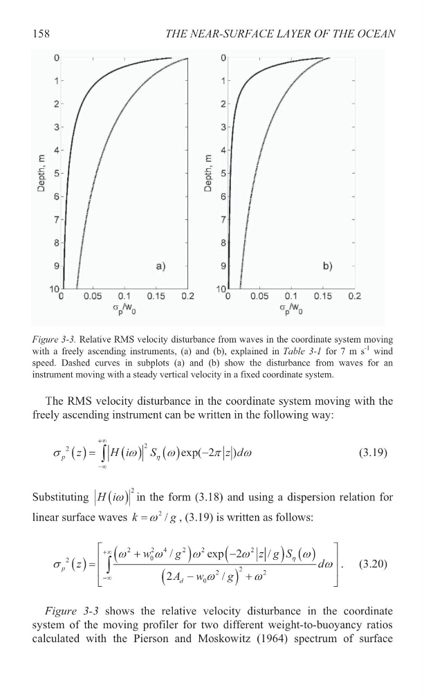
Figure 3-3. Relative RMS velocity disturbance from waves in the coordinate system moving
with a freely ascending instruments, (a) and (b), explained in Table 3-1 for 7 m s
-1 wind
speed. Dashed curves in subplots (a) and (b) show the disturbance from waves for an
instrument moving with a steady vertical velocity in a fixed coordinate system.
The RMS velocity disturbance in the coordinate system moving with the
freely ascending instrument can be written in the following way:
2
2
exp( 2
)
p
z
H i
S
z d
K
V
Z
Z
S
Z
f
f
³
(3.19)
Substituting
2
H iZ in the form (3.18) and using a dispersion relation for
linear surface waves
2 /
k
g
Z
, (3.19) is written as follows:
2
2 4
2
2
2
0
2
2
2
2
0
/
exp 2
/
2
/
p
d
w
g
z g S
z
d
A w
g
K
Z
Z
Z
Z
Z
V
Z
Z
Z
f
f
ª
º
«
»
«
»
¬
¼
³
. (3.20)
Figure 3-3 shows the relative velocity disturbance in the coordinate
system of the moving profiler for two different weight-to-buoyancy ratios
calculated with the Pierson and Moskowitz (1964) spectrum of surface
158