

Satellite Oceanography for Ocean Forecasting
27
At the surface, P is equal to p g 11, where 11 is the dynamic topography (sea level
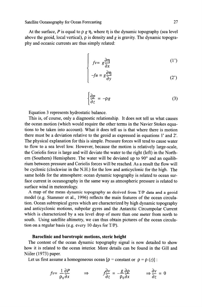
above the geoid, local vertical), p is density and g is gravity. The dynamic topography and oceanic currents are thus simply re1ated:
fv= i 11
ax
-fu = i 11
ay
{ a p = -pg
az
Equation 3 represents hydrostatic balance.
(l ')
(2')
(3)
This is, of course, only a diagnostic relationship. It does not tell us what causes
the ocean motion (which would require the other terms in the Navier Stokes equations to be taken into account). What it does tell us is that where there is motion
there must be a deviation relative to the geoid as expressed in equations l' and 2'.
The physical explanation for this is simple. Pressure forces will tend to cause water
to flow to asea 1eve1 10w. However, because the motion is re1ative1y 1arge-sca1e,
the Coriolis force is large and will deviate the water to the right (left) in the Northern (Southern) Hemisphere. The water will be deviated up to 90° and an equilibrium between pressure and Coriolis forces will be reached. As a result the flow will
be cyclonic (clockwise in the N.R.) for the low and anticyclonic for the high. The
same holds for the atmosphere: ocean dynamic topography is related to ocean surface current in oceanography in the same way as atmospheric pressure is related to
surf ace wind in meteorology.
A map of the mean dynamic topography as derived from TIP data and a geoid
model (e.g. Stammer et al., 1996) reflects the main features of the ocean circulation. Ocean subtropical gyres which are characterized by high dynamic topography
and anticyclonic motions, subpolar gyres and the Antarctic Circumpo1ar Current
which is characterized by asea leve1 drop of more than one meter from north to
south. Using satellite altimetry, we can thus obtain pictures of the ocean circulation on a regular basis (e.g. every 10 days for TIP).
Baroclinic and barotropic motions, steric height
The content of the ocean dynamic topography signal is now detailed to show
how it is re1ated to the ocean interior. More detai1s can be found in the Gill and
Niiler (1973) paper.
Let us first assume a homogeneous ocean [p = constant or p = p (z)] :
~av = O
az
27
At the surface, P is equal to p g 11, where 11 is the dynamic topography (sea level
above the geoid, local vertical), p is density and g is gravity. The dynamic topography and oceanic currents are thus simply re1ated:
fv= i 11
ax
-fu = i 11
ay
{ a p = -pg
az
Equation 3 represents hydrostatic balance.
(l ')
(2')
(3)
This is, of course, only a diagnostic relationship. It does not tell us what causes
the ocean motion (which would require the other terms in the Navier Stokes equations to be taken into account). What it does tell us is that where there is motion
there must be a deviation relative to the geoid as expressed in equations l' and 2'.
The physical explanation for this is simple. Pressure forces will tend to cause water
to flow to asea 1eve1 10w. However, because the motion is re1ative1y 1arge-sca1e,
the Coriolis force is large and will deviate the water to the right (left) in the Northern (Southern) Hemisphere. The water will be deviated up to 90° and an equilibrium between pressure and Coriolis forces will be reached. As a result the flow will
be cyclonic (clockwise in the N.R.) for the low and anticyclonic for the high. The
same holds for the atmosphere: ocean dynamic topography is related to ocean surface current in oceanography in the same way as atmospheric pressure is related to
surf ace wind in meteorology.
A map of the mean dynamic topography as derived from TIP data and a geoid
model (e.g. Stammer et al., 1996) reflects the main features of the ocean circulation. Ocean subtropical gyres which are characterized by high dynamic topography
and anticyclonic motions, subpolar gyres and the Antarctic Circumpo1ar Current
which is characterized by asea leve1 drop of more than one meter from north to
south. Using satellite altimetry, we can thus obtain pictures of the ocean circulation on a regular basis (e.g. every 10 days for TIP).
Baroclinic and barotropic motions, steric height
The content of the ocean dynamic topography signal is now detailed to show
how it is re1ated to the ocean interior. More detai1s can be found in the Gill and
Niiler (1973) paper.
Let us first assume a homogeneous ocean [p = constant or p = p (z)] :
~av = O
az