

Primitive Equation Modelling ofPlankton Ecosystems
L09 1O[cells/ m2j - r - - - - -- - - - - - - - - - - - - - - - - ,
10
9
8
7
6
5
Year 1
~
u
ÎO
::;:
~
Year 2
~
~
Year 3
"'
::;:
' "
403
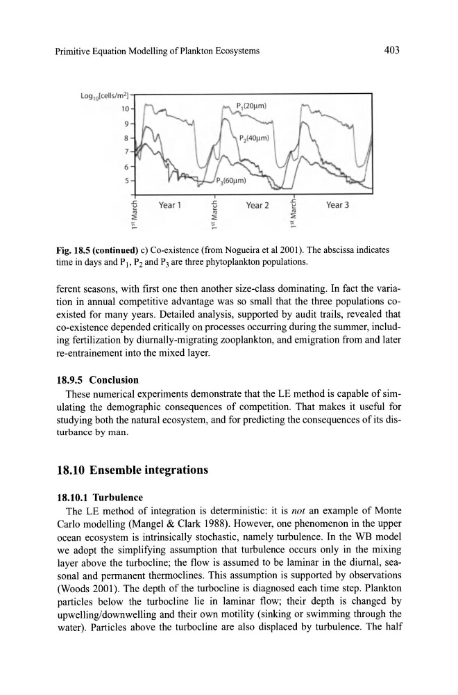
Fig. 18.5 (continued) c) Co-existence (from Nogueira et al 2001). The abscissa indicates
time in days and Pj, P 2 and P 3 are three phytoplankton populations.
ferent seasons, with first one then another size-cIass dominating. In fact the variation in annual competitive advantage was so small that the three populations coexisted for many years. Detailed analysis, supported by audit trails, revealed that
co-existence depended critically on processes occurring during the summer, incIuding fertilization by diumally-migrating zooplankton, and emigration from and later
re-entrainement into the mixed layer.
18.9.5 Conclusion
These numerical experiments demonstrate that the LE method is capable of simulating the demographic consequences of competition. That makes it useful for
studying both the natural ecosystem, and for predicting the consequences of its disturbance by man.
18.10 Ensemble integrations
18.10.1 Turbulence
The LE method of integration is deterministic: it is not an example of Monte
Carlo modelling (Mangel & Clark 1988). However, one phenomenon in the upper
ocean ecosystem is intrinsically stochastic, namely turbulence. In the WB model
we adopt the simplifying assumption that turbulence occurs only in the mixing
layer above the turbocline; the flow is assumed to be laminar in the diumal, seasonal and permanent thermocIines. This assumption is supported by observations
(Woods 2001). The depth of the turbocline is diagnosed each time step. Plankton
particIes below the turbocIine lie in laminar flow; their depth is changed by
upwelling/downwelling and their own motility (sinking or swimming through the
water). Particles above the turboc\ine are also displaced by turbulence. The half
L09 1O[cells/ m2j - r - - - - -- - - - - - - - - - - - - - - - - ,
10
9
8
7
6
5
Year 1
~
u
ÎO
::;:
~
Year 2
~
~
Year 3
"'
::;:
' "
403
Fig. 18.5 (continued) c) Co-existence (from Nogueira et al 2001). The abscissa indicates
time in days and Pj, P 2 and P 3 are three phytoplankton populations.
ferent seasons, with first one then another size-cIass dominating. In fact the variation in annual competitive advantage was so small that the three populations coexisted for many years. Detailed analysis, supported by audit trails, revealed that
co-existence depended critically on processes occurring during the summer, incIuding fertilization by diumally-migrating zooplankton, and emigration from and later
re-entrainement into the mixed layer.
18.9.5 Conclusion
These numerical experiments demonstrate that the LE method is capable of simulating the demographic consequences of competition. That makes it useful for
studying both the natural ecosystem, and for predicting the consequences of its disturbance by man.
18.10 Ensemble integrations
18.10.1 Turbulence
The LE method of integration is deterministic: it is not an example of Monte
Carlo modelling (Mangel & Clark 1988). However, one phenomenon in the upper
ocean ecosystem is intrinsically stochastic, namely turbulence. In the WB model
we adopt the simplifying assumption that turbulence occurs only in the mixing
layer above the turbocline; the flow is assumed to be laminar in the diumal, seasonal and permanent thermocIines. This assumption is supported by observations
(Woods 2001). The depth of the turbocline is diagnosed each time step. Plankton
particIes below the turbocIine lie in laminar flow; their depth is changed by
upwelling/downwelling and their own motility (sinking or swimming through the
water). Particles above the turboc\ine are also displaced by turbulence. The half