

ENSO Predictions with Coupled Ocean Atmosphere Models
321
N
T'(x, t) = L an(t)En(x)
(1)
n = 1
N
't'(x, t) = L ~n(t)Fn(x)
(2)
n = 1
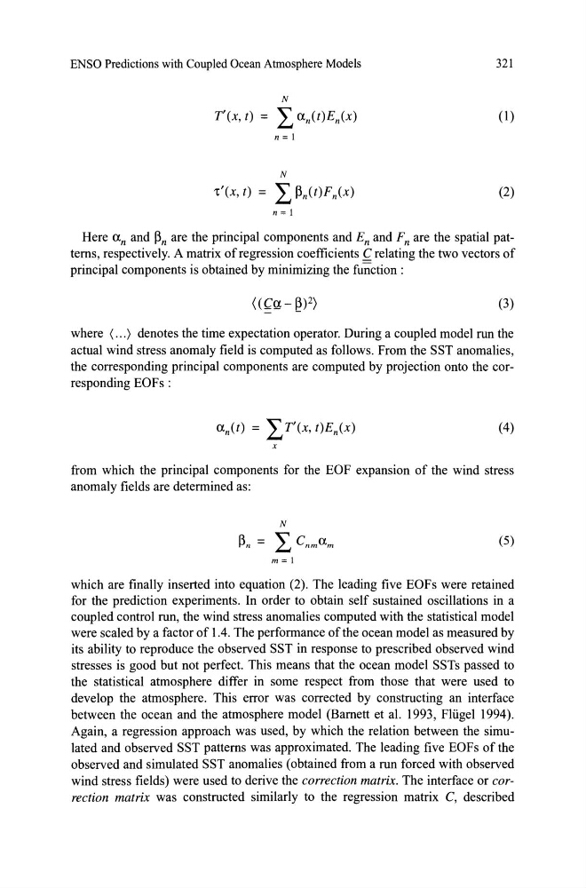
Here an and ~n are the principal components and En and Fn are the spatial pattems, respectively. A matrix of regression coefficients f relating the two vectors of
principal components is obtained by minimizing the function :
(3)
where < ... ) denotes the time expectation operator. During a coupled model run the
actual wind stress anomaly field is computed as follows. From the SST anomalies,
the corresponding principal components are computed by projection onto the corresponding EOFs :
(4)
x
from which the principal components for the EOF expansion of the wind stress
anomaly fields are determined as:
(5)
m = 1
which are finally inserted into equation (2). The leading five EOFs were retained
for the prediction experiments. In order to obtain self sustained oscillations in a
coupled control run' the wind stress anomalies computed with the statistical model
were scaled by a factor of 1.4. The performance ofthe ocean model as measured by
its ability to reproduce the observed SST in response to prescribed observed wind
stresses is good but not perfect. This means that the ocean model SSTs passed to
the statistical atmosphere differ in some respect from those that were used to
develop the atmosphere. This error was corrected by constructing an interface
between the ocean and the atmosphere model (Bamett et al. 1993, Fliigel 1994).
Again, a regression approach was used, by which the relation between the simulated and observed SST pattems was approximated. The leading five EOFs of the
observed and simulated SST anomalies (obtained from a run forced with observed
wind stress fields) were used to derive the correction matrix. The interface or correction matrix was constructed similarly to the regression matrix C, described
321
N
T'(x, t) = L an(t)En(x)
(1)
n = 1
N
't'(x, t) = L ~n(t)Fn(x)
(2)
n = 1
Here an and ~n are the principal components and En and Fn are the spatial pattems, respectively. A matrix of regression coefficients f relating the two vectors of
principal components is obtained by minimizing the function :
(3)
where < ... ) denotes the time expectation operator. During a coupled model run the
actual wind stress anomaly field is computed as follows. From the SST anomalies,
the corresponding principal components are computed by projection onto the corresponding EOFs :
(4)
x
from which the principal components for the EOF expansion of the wind stress
anomaly fields are determined as:
(5)
m = 1
which are finally inserted into equation (2). The leading five EOFs were retained
for the prediction experiments. In order to obtain self sustained oscillations in a
coupled control run' the wind stress anomalies computed with the statistical model
were scaled by a factor of 1.4. The performance ofthe ocean model as measured by
its ability to reproduce the observed SST in response to prescribed observed wind
stresses is good but not perfect. This means that the ocean model SSTs passed to
the statistical atmosphere differ in some respect from those that were used to
develop the atmosphere. This error was corrected by constructing an interface
between the ocean and the atmosphere model (Bamett et al. 1993, Fliigel 1994).
Again, a regression approach was used, by which the relation between the simulated and observed SST pattems was approximated. The leading five EOFs of the
observed and simulated SST anomalies (obtained from a run forced with observed
wind stress fields) were used to derive the correction matrix. The interface or correction matrix was constructed similarly to the regression matrix C, described