

Forecasting Wind-driven Ocean Waves
275
the growth of longer waves. Therefore, the very short wave scales are not resolved
in the WAM model. It is then consistent to assume that there is always a minimum
spectral energy level, which can be parametrised in terms of the grid size, the time
step and the wind speed. When a cold start is made the model is initialised at this
level.
14.3.1 The energy balance
The first applications ofthe WAM model concemed the ideali sed cases discussed
in the previous section. It is instructive here to consider the case of duration-limited
growth. The phenomenology of this type of growth was discussed above: a peaked
spectrum; a peak that moves to the left when duration increases; overshoot at high
frequencies; and an approach to a fully grown stage in which the spectrum does not
change anymore. AII of these features have been reproduced (Komen, Hasselmann
and Hasselmann, 1984). An analysis of these results has greatly improved our
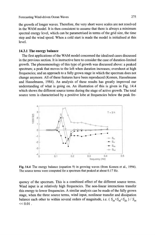
understanding of what is going ono An illustration of this is given in Fig. 14.4
which shows the different source terms during the stage of active growth. The total
source term is characterised by a positive lobe at frequencies below the peak fre4
3
(j) 2
o
o
;?
o
•
-1
-Q- S.,
-2
S nl
S'"
-3
~ S to,
-4 o
0.1
0.2
0.3
0.4
0.5
frequency (Hz)
Fig. 14.4 The energy balance (equation 9) in growing waves (from Komen et al., 1994).
The source terms were computed for a spectrum that peaked at about 0.17 Hz.
quency of the spectrum. This is a combined effect of the different source terms.
Wind input is at relatively high frequencies. The non-linear interactions transfer
this energy to lower frequencies . A similar analysis can be made ofthe fully grown
stage, when the three source terms, wind input, non linear transfer and dissipation
balance each other to within several orders of magnitude, i.e. ( Sin +Snl+Sds ) / Sin
« 0.01 .
275
the growth of longer waves. Therefore, the very short wave scales are not resolved
in the WAM model. It is then consistent to assume that there is always a minimum
spectral energy level, which can be parametrised in terms of the grid size, the time
step and the wind speed. When a cold start is made the model is initialised at this
level.
14.3.1 The energy balance
The first applications ofthe WAM model concemed the ideali sed cases discussed
in the previous section. It is instructive here to consider the case of duration-limited
growth. The phenomenology of this type of growth was discussed above: a peaked
spectrum; a peak that moves to the left when duration increases; overshoot at high
frequencies; and an approach to a fully grown stage in which the spectrum does not
change anymore. AII of these features have been reproduced (Komen, Hasselmann
and Hasselmann, 1984). An analysis of these results has greatly improved our
understanding of what is going ono An illustration of this is given in Fig. 14.4
which shows the different source terms during the stage of active growth. The total
source term is characterised by a positive lobe at frequencies below the peak fre4
3
(j) 2
o
o
;?
o
•
-1
-Q- S.,
-2
S nl
S'"
-3
~ S to,
-4 o
0.1
0.2
0.3
0.4
0.5
frequency (Hz)
Fig. 14.4 The energy balance (equation 9) in growing waves (from Komen et al., 1994).
The source terms were computed for a spectrum that peaked at about 0.17 Hz.
quency of the spectrum. This is a combined effect of the different source terms.
Wind input is at relatively high frequencies. The non-linear interactions transfer
this energy to lower frequencies . A similar analysis can be made ofthe fully grown
stage, when the three source terms, wind input, non linear transfer and dissipation
balance each other to within several orders of magnitude, i.e. ( Sin +Snl+Sds ) / Sin
« 0.01 .