

Ensembles, Forecasts and Predictability
Inlluence 01
/
Initial Conditions
I
I
Start 1 Week 1 Months
3 Months
Influence 01
Bundary Conditions
145
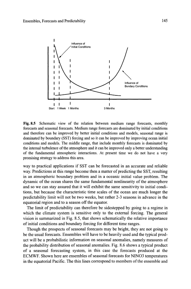
Fig. 8.5 Schematic view of the re1ation between medium range forecasts, monthly
forecasts and seasonal forecasts. Medium range forecasts are dominated by initial conditions
and therefore can be improved by better initial conditions and models, seasonal range is
dominated by boundary (SST) forcing and so it can be improved by improving ocean initial
conditions and models. The middle range, that include monthly forecasts is dominated by
the internal turbulence of the atmosphere and it can be improved only a better understanding
of the fundamental atmospheric interactions. At present time we do not have a very
promising strategy to address this area.
way to practical applications if SST can be forecasted in an accurate and reliable
way. Predictions at this range become then a matter of predicting the SST, resulting
in an atmospheric boundary problem and in a oceanic initial value prob1em. The
dynamic of the ocean shares the same fundamental nonlinearity of the atmosphere
and so we can stay assured that it will exhibit the same sensitivity to initial conditions, but because the characteristic time scales of the ocean are much longer the
predictability limit will not be two weeks, but rather 2-3 seasons in advance in the
equatorial region and to a season off the equator.
The limit of predictability can therefore be sidestepped by going to a regime in
which the climate system is sensitive only to the external forcing. The general
vision is summarized in Fig. 8.5, that shows schematically the relative importance
of initial conditions and boundary forcing for different time ranges.
Though the prospects of seasonal forecasts may be bright, they are not going to
be the usual forecasts. Ensembles will have to be heavily used and the typical product will be a probabilistic information on seasonal anomalies, namely measures of
the probability distribution of seasonal anomalies. Fig. 8.6 shows a typical product
of a seasonal forecasting system, in this case the forecasts produced at the
ECMWF. Shown here are ensembles of seasonal forecasts for NIN03 temperatures
in the equatorial Pacific. The thin lines correspond to members ofthe ensemble and
Inlluence 01
/
Initial Conditions
I
I
Start 1 Week 1 Months
3 Months
Influence 01
Bundary Conditions
145
Fig. 8.5 Schematic view of the re1ation between medium range forecasts, monthly
forecasts and seasonal forecasts. Medium range forecasts are dominated by initial conditions
and therefore can be improved by better initial conditions and models, seasonal range is
dominated by boundary (SST) forcing and so it can be improved by improving ocean initial
conditions and models. The middle range, that include monthly forecasts is dominated by
the internal turbulence of the atmosphere and it can be improved only a better understanding
of the fundamental atmospheric interactions. At present time we do not have a very
promising strategy to address this area.
way to practical applications if SST can be forecasted in an accurate and reliable
way. Predictions at this range become then a matter of predicting the SST, resulting
in an atmospheric boundary problem and in a oceanic initial value prob1em. The
dynamic of the ocean shares the same fundamental nonlinearity of the atmosphere
and so we can stay assured that it will exhibit the same sensitivity to initial conditions, but because the characteristic time scales of the ocean are much longer the
predictability limit will not be two weeks, but rather 2-3 seasons in advance in the
equatorial region and to a season off the equator.
The limit of predictability can therefore be sidestepped by going to a regime in
which the climate system is sensitive only to the external forcing. The general
vision is summarized in Fig. 8.5, that shows schematically the relative importance
of initial conditions and boundary forcing for different time ranges.
Though the prospects of seasonal forecasts may be bright, they are not going to
be the usual forecasts. Ensembles will have to be heavily used and the typical product will be a probabilistic information on seasonal anomalies, namely measures of
the probability distribution of seasonal anomalies. Fig. 8.6 shows a typical product
of a seasonal forecasting system, in this case the forecasts produced at the
ECMWF. Shown here are ensembles of seasonal forecasts for NIN03 temperatures
in the equatorial Pacific. The thin lines correspond to members ofthe ensemble and