

134 Antonio Navarra
Dispersion of trajectories in Ihe Lorenz system
20r----.----.----,-----,----.----.----.----,----~
10
o
- 10
-20~--~----~----L---~-----L----~----L---~----~
-5
O
5
10
15
20
25
30
35
40
Dispersion for Ihe linear case
20 ,----,---,----,----,----,----,----,----.---.
10
-
o
- 10
...
-20 ~---L----~--~----L----L----L----L----L---~
-5
O
5
10
15
20
25
30
35
40
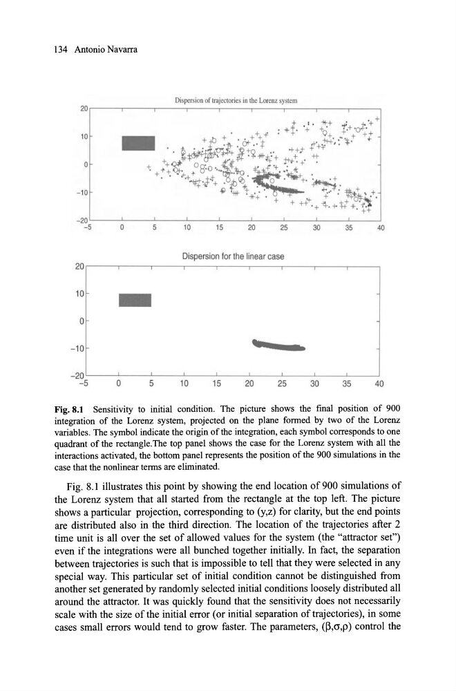
Fig. 8.1 Sensitivity to initial condition. The picture shows the final posltlon of 900
integration of the Lorenz system, projected on the plane formed by two of the Lorenz
variables. The symbol indicate the origin of the integration, each symbol corresponds to one
quadrant of the rectangle.The top panel shows the case for the Lorenz system with all the
interactions activated, the bottom panel represents the position of the 900 simulations in the
case that the nonlinear terms are eliminated.
Fig. 8.1 illustrates this point by showing the end location of 900 simulations of
the Lorenz system that ali started from the rectangle at the top left. The picture
shows a particular projection, corresponding to (y,z) for clarity, but the end points
are distributed also in the third direction. The location of the trajectories after 2
time unit is ali over the set of allowed values for the system (the "attractor set")
even if the integrations were ali bunched together initially. In fact, the separation
between trajectories is such that is impossible to tell that they were selected in any
special way. This particular set of initial condition cannot be distinguished from
another set generated by randomly selected initial conditions loosely distributed ali
around the attractor. It was quickly found that the sensitivity does not necessarily
scale with the size ofthe initial error (or initial separation oftrajectories), in some
cases small errors would tend to grow faster. The parameters, (~,cr,p) control the
Dispersion of trajectories in Ihe Lorenz system
20r----.----.----,-----,----.----.----.----,----~
10
o
- 10
-20~--~----~----L---~-----L----~----L---~----~
-5
O
5
10
15
20
25
30
35
40
Dispersion for Ihe linear case
20 ,----,---,----,----,----,----,----,----.---.
10
-
o
- 10
...
-20 ~---L----~--~----L----L----L----L----L---~
-5
O
5
10
15
20
25
30
35
40
Fig. 8.1 Sensitivity to initial condition. The picture shows the final posltlon of 900
integration of the Lorenz system, projected on the plane formed by two of the Lorenz
variables. The symbol indicate the origin of the integration, each symbol corresponds to one
quadrant of the rectangle.The top panel shows the case for the Lorenz system with all the
interactions activated, the bottom panel represents the position of the 900 simulations in the
case that the nonlinear terms are eliminated.
Fig. 8.1 illustrates this point by showing the end location of 900 simulations of
the Lorenz system that ali started from the rectangle at the top left. The picture
shows a particular projection, corresponding to (y,z) for clarity, but the end points
are distributed also in the third direction. The location of the trajectories after 2
time unit is ali over the set of allowed values for the system (the "attractor set")
even if the integrations were ali bunched together initially. In fact, the separation
between trajectories is such that is impossible to tell that they were selected in any
special way. This particular set of initial condition cannot be distinguished from
another set generated by randomly selected initial conditions loosely distributed ali
around the attractor. It was quickly found that the sensitivity does not necessarily
scale with the size ofthe initial error (or initial separation oftrajectories), in some
cases small errors would tend to grow faster. The parameters, (~,cr,p) control the