

372
Equatorial Dynamics of the Thermocline: The Equatorial Undercurrent
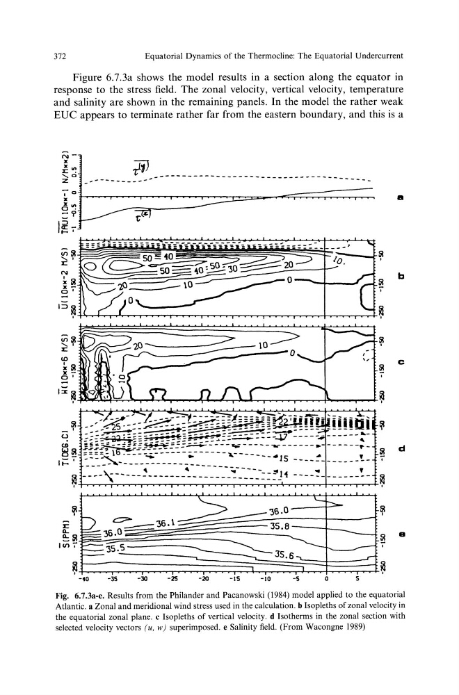
Figure 6.7.3a shows the model results in a section along the equator in
response to the stress field. The zonal velocity, vertical velocity, temperature
and salinity are shown in the remaining panels. In the model the rather weak
EUC appears to terminate rather far from the eastern boundary, and this is a
NX
x.,
:z::.
'-0
z
;tiJ
,~---------~-------------------------------------~~~~~~~~~~~~~~~~~~~~~~~~~~~----~ :z::
N
~51
xol
~~
:z:: """-~'~'
U)
~51 X -
ol
-10
-35
-JO
-25
-20
-15
-JO
-s
0
5
•
5I I
!!!
b
I
~
5I I
!!!
c
I
iii I
~
5I
d
i
~ I
:jl
!!! •
I
~
Fig. 6.7.3a-e. Results from the Philander and Pacanowski (1984) model applied to the equatorial
Atlantic. a Zonal and meridional wind stress used in the calculation. b Isopleths of zonal velocity in
the equatorial zonal plane. c Isopleths of vertical velocity. d Isotherms in the zonal section with
selected velocity vectors (u, w) superimposed. e Salinity field. (From Wacongne 1989)
Equatorial Dynamics of the Thermocline: The Equatorial Undercurrent
Figure 6.7.3a shows the model results in a section along the equator in
response to the stress field. The zonal velocity, vertical velocity, temperature
and salinity are shown in the remaining panels. In the model the rather weak
EUC appears to terminate rather far from the eastern boundary, and this is a
NX
x.,
:z::.
'-0
z
;tiJ
,~---------~-------------------------------------~~~~~~~~~~~~~~~~~~~~~~~~~~~----~ :z::
N
~51
xol
~~
:z:: """-~'~'
U)
~51 X -
ol
-10
-35
-JO
-25
-20
-15
-JO
-s
0
5
•
5I I
!!!
b
I
~
5I I
!!!
c
I
iii I
~
5I
d
i
~ I
:jl
!!! •
I
~
Fig. 6.7.3a-e. Results from the Philander and Pacanowski (1984) model applied to the equatorial
Atlantic. a Zonal and meridional wind stress used in the calculation. b Isopleths of zonal velocity in
the equatorial zonal plane. c Isopleths of vertical velocity. d Isotherms in the zonal section with
selected velocity vectors (u, w) superimposed. e Salinity field. (From Wacongne 1989)