

y
Effect of Entrainment
25+--+--+--+--~-+--~~--~~-+
20
15
10
0 o,_
367
20
1.5
y
10
05
b 0 0 ..j=::c,__,_.::::::OO..~+---f:c,._+--+--->~+---+---+
00
02
04
06
0.8
X
X
X
X
X
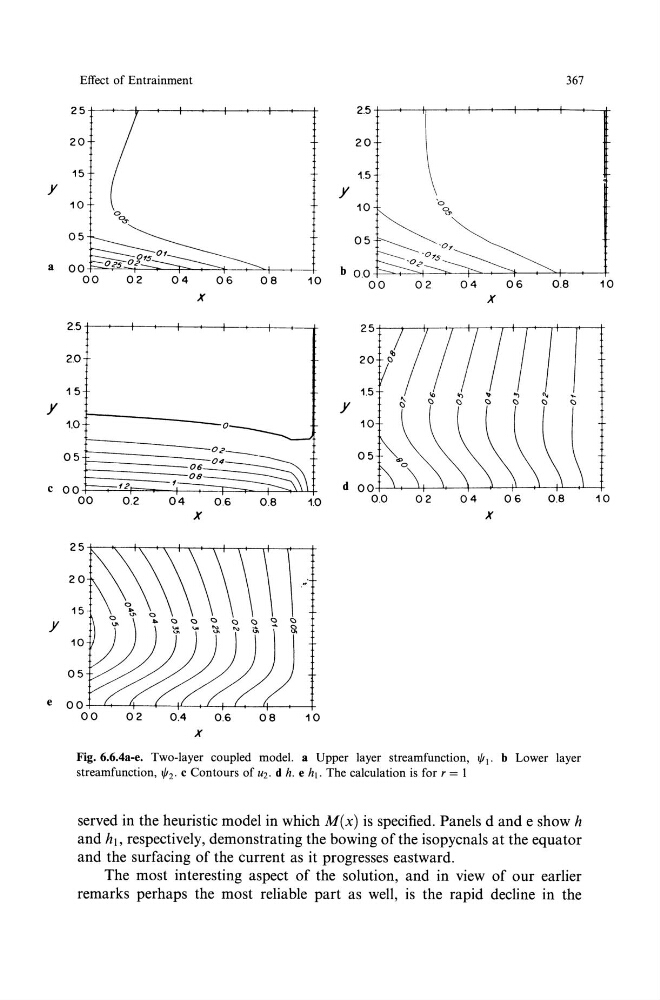
Fig. 6.6.4a-e. Two-layer coupled model. a Upper layer streamfunction, 1/t 1 • b Lower layer
streamfunction, 1/12 . c Contours of u2. d h. e ht. The calculation is for r = I
served in the heuristic model in which M(x) is specified. Panels d and e show h
and h,, respectively, demonstrating the bowing of the isopycnals at the equator
and the surfacing of the current as it progresses eastward.
The most interesting aspect of the solution, and in view of our earlier
remarks perhaps the most reliable part as well, is the rapid decline in the
10
Effect of Entrainment
25+--+--+--+--~-+--~~--~~-+
20
15
10
0 o,_
367
20
1.5
y
10
05
b 0 0 ..j=::c,__,_.::::::OO..~+---f:c,._+--+--->~+---+---+
00
02
04
06
0.8
X
X
X
X
X
Fig. 6.6.4a-e. Two-layer coupled model. a Upper layer streamfunction, 1/t 1 • b Lower layer
streamfunction, 1/12 . c Contours of u2. d h. e ht. The calculation is for r = I
served in the heuristic model in which M(x) is specified. Panels d and e show h
and h,, respectively, demonstrating the bowing of the isopycnals at the equator
and the surfacing of the current as it progresses eastward.
The most interesting aspect of the solution, and in view of our earlier
remarks perhaps the most reliable part as well, is the rapid decline in the
10