

360
Equatorial Dynamics of the Thermocline: The Equatorial Undercurrent
P1
tf*
I I
---.
I
~lo
v2 h2
~
2
I I
---.
IIi
p
l~
Y=O
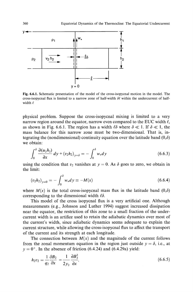
Fig. 6.6.1. Schematic presentation of the model of the cross-isopycnal motion in the model. The
cross-isopycnal flux is limited to a narrow zone of half-width [J£ within the undercurrent of halfwidth£
physical problem. Suppose the cross-isopycnal mixing is limited to a very
narrow region around the equator, narrow even compared to the EUC width£,
as shown in Fig. 6.6.1. The region has a width f(j where (j « 1. If (j « 1, the
mass balance for this narrow zone must be two-dimensional. That is, integrating the (nondimensional) continuity equation over the latitude band (O,b)
we obtain:
1 b a(uzhz)
1b
- - - dy + (vzhz)y=b = -
w.dy
0
~
0
(6.6.3)
using the condition that v2 vanishes at y = 0. As (j goes to zero, we obtain in
the limit:
(vzhz)y=O = -1b w.dy = -M(x)
( 6.6.4)
where M(x) is the total cross-isopycnal mass flux in the latitude band (O,b)
corresponding to the dimensional width£().
This model of the cross isopycnal flux is a very artificial one. Although
measurements (e.g., Johnson and Luther 1994) suggest increased dissipation
near the equator, the restriction of this zone to a small fraction of the undercurrent width is an artifice used to retain the adiabatic dynamics over most of
the current's width, since adiabatic dynamics seems adequate to explain the
current structure, while allowing the cross-isopycnal flux to affect the transport
of the current and its strength at each longitude.
The connection between M(x) and the magnitude of the current follows
from the zonal momentum equation in the region just outside y = (), i.e., at
y = o+. In the absence of friction (6.4.24) and (6.4.29a) yield:
(6.6.5)
Equatorial Dynamics of the Thermocline: The Equatorial Undercurrent
P1
tf*
I I
---.
I
~lo
v2 h2
~
2
I I
---.
IIi
p
l~
Y=O
Fig. 6.6.1. Schematic presentation of the model of the cross-isopycnal motion in the model. The
cross-isopycnal flux is limited to a narrow zone of half-width [J£ within the undercurrent of halfwidth£
physical problem. Suppose the cross-isopycnal mixing is limited to a very
narrow region around the equator, narrow even compared to the EUC width£,
as shown in Fig. 6.6.1. The region has a width f(j where (j « 1. If (j « 1, the
mass balance for this narrow zone must be two-dimensional. That is, integrating the (nondimensional) continuity equation over the latitude band (O,b)
we obtain:
1 b a(uzhz)
1b
- - - dy + (vzhz)y=b = -
w.dy
0
~
0
(6.6.3)
using the condition that v2 vanishes at y = 0. As (j goes to zero, we obtain in
the limit:
(vzhz)y=O = -1b w.dy = -M(x)
( 6.6.4)
where M(x) is the total cross-isopycnal mass flux in the latitude band (O,b)
corresponding to the dimensional width£().
This model of the cross isopycnal flux is a very artificial one. Although
measurements (e.g., Johnson and Luther 1994) suggest increased dissipation
near the equator, the restriction of this zone to a small fraction of the undercurrent width is an artifice used to retain the adiabatic dynamics over most of
the current's width, since adiabatic dynamics seems adequate to explain the
current structure, while allowing the cross-isopycnal flux to affect the transport
of the current and its strength at each longitude.
The connection between M(x) and the magnitude of the current follows
from the zonal momentum equation in the region just outside y = (), i.e., at
y = o+. In the absence of friction (6.4.24) and (6.4.29a) yield:
(6.6.5)