

352
Equatorial Dynamics of the Thermocline: The Equatorial Undercurrent
y•2S r--------------r-r------.-----~,~--r
a
I
I
i
i
,
,
y=o 1---.--..--.... --.---i>----r--r---T"""---r--+- u,h, fj
0
.5
u,h,
~
0
.5
4.0
c
i
i
y•2S r-------------~n---~--~-------.
i
I
!
/
,
-
-
. . -,
-
-
,
I
I
u,h, Jl!
.,
0
s
4.0
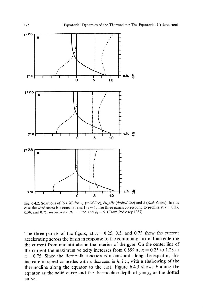
Fig. 6.4.2. Solutions of (6.4.26) for u2 (solid line), 8u2/8y (dashed line) and h (dash-dotted). In this
case the wind stress is a constant and r 12 = I. The three panels correspond to profiles at x = 0.25,
0.50, and 0.75, respectively. B0 = 1.265 and Y2 = 5. (From Pedlosky 1987)
The three panels of the figure, at x = 0.25, 0.5, and 0.75 show the current
accelerating across the basin in response to the continuing flux of fluid entering
the current from midlatitudes in the interior of the gyre. On the center line of
the current the maximum velocity increases from 0.899 at x = 0.25 to 1.28 at
x = 0.75. Since the Bernoulli function is a constant along the equator, this
increase in speed coincides with a decrease in h, i.e., with a shallowing of the
thermocline along the equator to the east. Figure 6.4.3 shows h along the
equator as the solid curve and the thermocline depth at y = Yn as the dotted
curve.
Equatorial Dynamics of the Thermocline: The Equatorial Undercurrent
y•2S r--------------r-r------.-----~,~--r
a
I
I
i
i
,
,
y=o 1---.--..--.... --.---i>----r--r---T"""---r--+- u,h, fj
0
.5
u,h,
~
0
.5
4.0
c
i
i
y•2S r-------------~n---~--~-------.
i
I
!
/
,
-
-
. . -,
-
-
,
I
I
u,h, Jl!
.,
0
s
4.0
Fig. 6.4.2. Solutions of (6.4.26) for u2 (solid line), 8u2/8y (dashed line) and h (dash-dotted). In this
case the wind stress is a constant and r 12 = I. The three panels correspond to profiles at x = 0.25,
0.50, and 0.75, respectively. B0 = 1.265 and Y2 = 5. (From Pedlosky 1987)
The three panels of the figure, at x = 0.25, 0.5, and 0.75 show the current
accelerating across the basin in response to the continuing flux of fluid entering
the current from midlatitudes in the interior of the gyre. On the center line of
the current the maximum velocity increases from 0.899 at x = 0.25 to 1.28 at
x = 0.75. Since the Bernoulli function is a constant along the equator, this
increase in speed coincides with a decrease in h, i.e., with a shallowing of the
thermocline along the equator to the east. Figure 6.4.3 shows h along the
equator as the solid curve and the thermocline depth at y = Yn as the dotted
curve.