

350
Equatorial Dynamics of the Thermocline: The Equatorial Undercurrent
This condition on Bo can be understood as follows. Suppose that the
western boundary current is fundamentally inertial, at least over the stretch
between y. and the equator. The Bernoulli function would therefore be conserved on each streamline in the boundary current as well as in the interior.
Consider the streamline given by ljJ = 1/1 0 . This streamline enters the boundary
layer at y = y. and, bifurcating, flows along the western wall to the equator. It
is the streamline which forms the inner edge of the boundary layer which then
emerges to flow along the equator. Its Bernoulli function is clearly the value Bo
that we are seeking to use in constructing the equatorial boundary layer. The
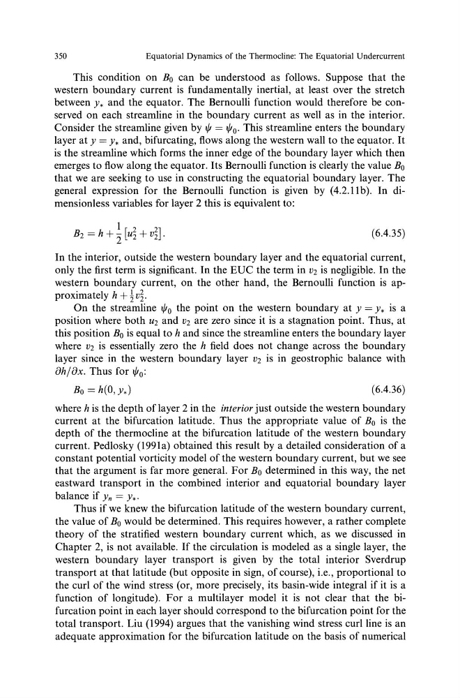
general expression for the Bernoulli function is given by ( 4.2.11 b). In dimensionless variables for layer 2 this is equivalent to:
(6.4.35)
In the interior, outside the western boundary layer and the equatorial current,
only the first term is significant. In the EUC the term in v2 is negligible. In the
western boundary current, on the other hand, the Bernoulli function is approximately h +!v~.
On the streamline 1/Jo the point on the western boundary at y = y. is a
position where both u2 and v2 are zero since it is a stagnation point. Thus, at
this position Bo is equal to h and since the streamline enters the boundary layer
where v2 is essentially zero the h field does not change across the boundary
layer since in the western boundary layer v2 is in geostrophic balance with
8h/8x. Thus for 1/1 0 :
Bo = h(O, y.)
(6.4.36)
where h is the depth of layer 2 in the interior just outside the western boundary
current at the bifurcation latitude. Thus the appropriate value of Bo is the
depth of the thermocline at the bifurcation latitude of the western boundary
current. Pedlosky (1991a) obtained this result by a detailed consideration of a
constant potential vorticity model of the western boundary current, but we see
that the argument is far more general. For Bo determined in this way, the net
eastward transport in the combined interior and equatorial boundary layer
balance if Yn = y •.
Thus if we knew the bifurcation latitude of the western boundary current,
the value of B0 would be determined. This requires however, a rather complete
theory of the stratified western boundary current which, as we discussed in
Chapter 2, is not available. If the circulation is modeled as a single layer, the
western boundary layer transport is given by the total interior Sverdrup
transport at that latitude (but opposite in sign, of course), i.e., proportional to
the curl of the wind stress (or, more precisely, its basin-wide integral if it is a
function of longitude). For a multilayer model it is not clear that the bifurcation point in each layer should correspond to the bifurcation point for the
total transport. Liu (1994) argues that the vanishing wind stress curl line is an
adequate approximation for the bifurcation latitude on the basis of numerical
Equatorial Dynamics of the Thermocline: The Equatorial Undercurrent
This condition on Bo can be understood as follows. Suppose that the
western boundary current is fundamentally inertial, at least over the stretch
between y. and the equator. The Bernoulli function would therefore be conserved on each streamline in the boundary current as well as in the interior.
Consider the streamline given by ljJ = 1/1 0 . This streamline enters the boundary
layer at y = y. and, bifurcating, flows along the western wall to the equator. It
is the streamline which forms the inner edge of the boundary layer which then
emerges to flow along the equator. Its Bernoulli function is clearly the value Bo
that we are seeking to use in constructing the equatorial boundary layer. The
general expression for the Bernoulli function is given by ( 4.2.11 b). In dimensionless variables for layer 2 this is equivalent to:
(6.4.35)
In the interior, outside the western boundary layer and the equatorial current,
only the first term is significant. In the EUC the term in v2 is negligible. In the
western boundary current, on the other hand, the Bernoulli function is approximately h +!v~.
On the streamline 1/Jo the point on the western boundary at y = y. is a
position where both u2 and v2 are zero since it is a stagnation point. Thus, at
this position Bo is equal to h and since the streamline enters the boundary layer
where v2 is essentially zero the h field does not change across the boundary
layer since in the western boundary layer v2 is in geostrophic balance with
8h/8x. Thus for 1/1 0 :
Bo = h(O, y.)
(6.4.36)
where h is the depth of layer 2 in the interior just outside the western boundary
current at the bifurcation latitude. Thus the appropriate value of Bo is the
depth of the thermocline at the bifurcation latitude of the western boundary
current. Pedlosky (1991a) obtained this result by a detailed consideration of a
constant potential vorticity model of the western boundary current, but we see
that the argument is far more general. For Bo determined in this way, the net
eastward transport in the combined interior and equatorial boundary layer
balance if Yn = y •.
Thus if we knew the bifurcation latitude of the western boundary current,
the value of B0 would be determined. This requires however, a rather complete
theory of the stratified western boundary current which, as we discussed in
Chapter 2, is not available. If the circulation is modeled as a single layer, the
western boundary layer transport is given by the total interior Sverdrup
transport at that latitude (but opposite in sign, of course), i.e., proportional to
the curl of the wind stress (or, more precisely, its basin-wide integral if it is a
function of longitude). For a multilayer model it is not clear that the bifurcation point in each layer should correspond to the bifurcation point for the
total transport. Liu (1994) argues that the vanishing wind stress curl line is an
adequate approximation for the bifurcation latitude on the basis of numerical