

148
Vertical Structure: Baroclinic Quasi-Geostrophic Models
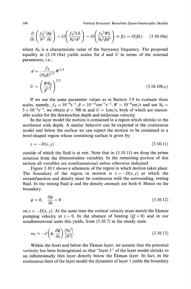
(3.10.10a)
where No is a characteristic value of the buoyancy frequency. The proposed
equality in (3.10.10a) yields scales ford and U in terms of the external
parameters, i.e.:
d =
fo
wl/3
(No/3)2/3
(
)
2/3
U= ;:~
(3.10.10b,c)
If we use the same parameter values as in Section 3.9 to evaluate these
scales, namely, fo = 10- 4 s-l, f3 = 10- 13 cm- 1 s-l, W = 10- 4 cmjs and use No=
5 x 10- 3 s- 1 , we obtain d = 700 m and U = lcmjs, both of which are reasonable scales for the thermocline depth and midocean velocity.
In the layer model the motion is contained in a region which shrinks to the
northwest with depth. A similar behavior can be expected in the continuous
model and below the surface we can expect the motion to be contained in a
bowl-shaped region whose containing surface is given by:
z = -D(x,y)
(3.10.11)
outside of which the fluid is at rest. Note that in (3.10.11) we drop the prime
notation from the dimensionless variables. In the remaining portion of this
section all variables are nondimensional unless otherwise indicated.
Figure 3.10.1 shows a schematic of the region in which motion takes place.
The boundary of the region in motion is z = -D(x, y) at which the
streamfunction and density must be continuous with the surrounding, resting
fluid. In the resting fluid t/1 and the density anomaly are both 0. Hence on the
boundary:
t/1 =0, ot/J = o
oz
(3.10.12)
on z = -D(x, y). At the same time the vertical velocity must match the Ekman
pumping velocity at z = 0. In the absence of heating (Q = 0) and in our
nondimensional units this yields, from (3.10.7) in the steady state:
(3.10.13)
Within the bowl and below the Ekman layer, we assume that the potential
vorticity has been homogenized so that "layer 1" of the layer model shrinks to
an infinitesimally thin layer directly below the Ekman layer. In fact, in the
continuous limit of the layer model the dynamics of layer 1 yields the boundary
Vertical Structure: Baroclinic Quasi-Geostrophic Models
(3.10.10a)
where No is a characteristic value of the buoyancy frequency. The proposed
equality in (3.10.10a) yields scales ford and U in terms of the external
parameters, i.e.:
d =
fo
wl/3
(No/3)2/3
(
)
2/3
U= ;:~
(3.10.10b,c)
If we use the same parameter values as in Section 3.9 to evaluate these
scales, namely, fo = 10- 4 s-l, f3 = 10- 13 cm- 1 s-l, W = 10- 4 cmjs and use No=
5 x 10- 3 s- 1 , we obtain d = 700 m and U = lcmjs, both of which are reasonable scales for the thermocline depth and midocean velocity.
In the layer model the motion is contained in a region which shrinks to the
northwest with depth. A similar behavior can be expected in the continuous
model and below the surface we can expect the motion to be contained in a
bowl-shaped region whose containing surface is given by:
z = -D(x,y)
(3.10.11)
outside of which the fluid is at rest. Note that in (3.10.11) we drop the prime
notation from the dimensionless variables. In the remaining portion of this
section all variables are nondimensional unless otherwise indicated.
Figure 3.10.1 shows a schematic of the region in which motion takes place.
The boundary of the region in motion is z = -D(x, y) at which the
streamfunction and density must be continuous with the surrounding, resting
fluid. In the resting fluid t/1 and the density anomaly are both 0. Hence on the
boundary:
t/1 =0, ot/J = o
oz
(3.10.12)
on z = -D(x, y). At the same time the vertical velocity must match the Ekman
pumping velocity at z = 0. In the absence of heating (Q = 0) and in our
nondimensional units this yields, from (3.10.7) in the steady state:
(3.10.13)
Within the bowl and below the Ekman layer, we assume that the potential
vorticity has been homogenized so that "layer 1" of the layer model shrinks to
an infinitesimally thin layer directly below the Ekman layer. In fact, in the
continuous limit of the layer model the dynamics of layer 1 yields the boundary