

Simulation of Oxygen Isotopes in a Global Ocean Model
679
high positive values in the subtropics, where evaporation dominates over precipitation, small negative
values in the equatorial trough region and high negative values in the mid- and high latitudes, where
precipitation dominates over evaporation. Excess
evaporation concentrates the less volatile isotopic
molecule IH 2
18 0 along with salinity, in agreement
with the positive 0p_E values (Craig and Gordon
1965).
The prescribed surface 0 18 0 field shows meridional gradients across the boundaries of the different regions given in Table I, in particular in the
North Atlantic at 25°N and in the Southern Ocean.
These meridonal gradients are reflected in the Ow
surface fluxes. But since the restoring is not very
stiff (t = 50 d), they are smeared out in the uppermost model layer by advection and diffusion processes, such that the simulated surface Ow fields look
rather smooth (Fig. 14). In comparison to Experiments A, Experiment B shows a less depleted net
surface fresh water flux in the Southern Ocean,
along with a much smaller meridional gradient.
Discussion
The advantage of restoring boundary conditions
over full flux boundary conditions is that the ocean
model can be run to equilibrium without flux adjustments. In a sense our approach is complementary
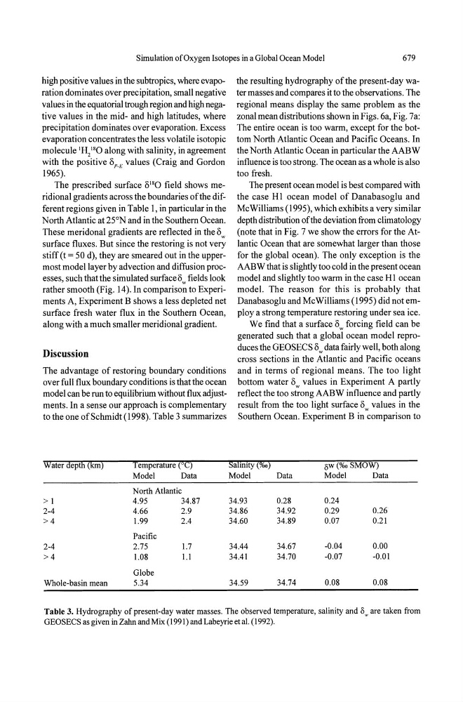
to the one of Schmidt (1998). Table 3 summarizes
Water depth (kill)
Temperature (0C)
Model
Data
North Atlantic
> 1
4.95
34.87
2-4
4.66
2.9
>4
1.99
2.4
Pacific
2-4
2.75
1.7
>4
1.08
1.1
Globe
Whole-basin mean
5.34
the resulting hydrography ofthe present-day water masses and compares it to the observations. The
regional means display the same problem as the
zonal mean distributions shown in Figs. 6a, Fig. 7a:
The entire ocean is too warm, except for the bottom North Atlantic Ocean and Pacific Oceans. In
the North Atlantic Ocean in particular the AABW
influence is too strong. The ocean as a whole is also
too fresh.
The present ocean model is best compared with
the case HI ocean model of Danabasoglu and
McWilliams (1995), which exhibits a very similar
depth distribution of the deviation from climatology
(note that in Fig. 7 we show the errors for the Atlantic Ocean that are somewhat larger than those
for the global ocean). The only exception is the
AABW that is slightly too cold in the present ocean
model and slightly too warm in the case HI ocean
model. The reason for this is probably that
Danabasoglu and McWilliams (1995) did not employ a strong temperature restoring under sea ice.
We find that a surface Ow forcing field can be
generated such that a global ocean model reproduces the GEOSECS Ow data fairly well, both along
cross sections in the Atlantic and Pacific oceans
and in terms of regional means. The too light
bottom water Ow values in Experiment A partly
reflect the too strong AABW influence and partly
result from the too light surface Ow values in the
Southern Ocean. Experiment B in comparison to
Sahmty (%0)
OW (%0 SMOW)
Model
Data
Model
Data
34.93
0.28
0.24
34.86
34.92
0.29
0.26
34.60
34.89
0.07
0.21
34.44
34.67
-0.04
0.00
34.41
34.70
-0.07
-0.01
34.59
34.74
0.08
0.08
Table 3. Hydrography of present-day water masses. The observed temperature, salinity and S,.. are taken from
GEOSECS as given in Zahn and Mix (1991) and Labeyrie et al. (1992).