

Metocean Extreme and Operating Conditions 3.6 Operational Criteria 65
Part A | 3.6
0
5
1 0
10%
20%
40%
5–10
Wind speed (m/s)
0–5
Hdg(from)
0
45
90 135 180 225 270 315 Sub. Total
2.5 18.61 3.33 7.92 4.89 2.51 1.15 0.94 0.73 40.09 40.09
7.5 0.09 9.59 26.17 7.05 3.27 2.20 0.95 0.56 50.53 90.61
12.5 0.07 1.90 6.07 0.21 0.30 0.21 0.26 0.12 9.13 99.74
17.5 0.01 0.01 0.02 0.02 0.02 0.06 0.05 0.02 0.19 99.93
22.5 0.00 0.01 0.00 0.00 0.02 0.00 0.01 0.01 0.04 99.98
27.5 0.00 0.00 0.00 0.00 0.01 0.00 0.00 0.01 0.02 99.99
32.5 0.00 0.00 0.00 0.00 0.00 0.00 0.00 0.01 0.01 100.00
37.5 0.00 0.00 0.00 0.00 0.00 0.00 0.00 0.00 0.00 100.00
19.38 14.83 40.18 12.17 6.12 3.61 2.25 1.45 100
100
19.38 34.22 74.40 86.57 92.69 96.30 98.55 100 100
100
Spd (m/s)
Sub.
Total
>10
30%
15
20
a) P (Spd = s)
b)
c)
Wind speed (m/s)
20
15
10
5
0
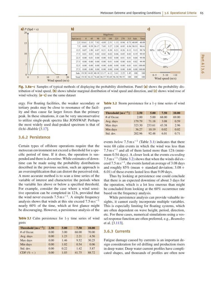
Fig. 3.8a–c Samples of typical methods of displaying the probability distribution. Panel (a) shows the probability distribution of wind speed, (b) shows tabular marginal distribution of wind speed and direction, and (c) shows wind rose of
wind velocity. (a–c) use the same dataset
ergy. For floating facilities, the weaker secondary or
tertiary peaks may be close to resonance of the facility and thus cause far larger forces than the primary
peak. In these situations, it can be very unconservative
to utilize single-peak spectra like JONSWAP. Perhaps
the most widely used dual-peaked spectrum is that of
Ochi–Hubble [3.17].
3.6.2 Persistence
Certain types of offshore operations require that the
metocean environment not exceed a threshold for a specific period of time. If it does, the operation is suspended and there is downtime. While estimates of downtime can be made using the probability distributions
described in the previous section, such an approach is
an oversimplification that can distort the perceived risk.
A more accurate method is to scan a time series of the
variable of interest and characterize the periods when
the variable lies above or below a specified threshold.
For example, consider the case where a wind sensitive operation can be completed in 12 h, provided that
the wind never exceeds 7:5 m s
1 . A simple frequency
analysis shows that winds at this site exceed 7:5 m s
1
nearly 60% of the time, which at first glance might
be discouraging. However, a persistence analysis of the
Table 3.1 Calm persistence for 1-y time series of wind
gusts
Threshold [m s 1 ] 2.50
5.00
7.50
10.00
# of Occur.
0.00
3.00
68.00
70.00
Avg. days
0.00
1.23
2.21
4.56
Max days
0.00
1.46
9.52
30.25
Min days
0.00
1.02
0.54
0.06
Std. dev.
0.00
0.22
1.42
5.87
CDF (% < )
0.00
1.03
41.75
88.72
Table 3.2 Storm persistence for a 1-y time series of wind
gusts
Threshold [m s 1 ]
2.50
5.00
7.50
10.00
# of Occur.
2.00
5.00
68.00
69.00
Avg. days
179.79
71.18
3.08
0.59
Max days
323.30
233.61
43.38
2.96
Min days
36.27
10.19
0.02
0.02
Std. dev.
202.96
92.48
6.01
0.71
events below 7:5 m s
1 (Table 3.1) indicates that there
were 68 calm events in which the wind was less than
7:5 m s
1 and all of them lasted more than 12 h (minimum 0.54 days). A closer look at the events exceeding
7:5 m s
1 (Table 3.2) shows that when the winds did exceed 7:5 m s
1 , the events lasted an average of 3.08 days
and roughly 85% (mean C standard deviation; 3:08 C
6:01) of these events lasted less than 9:09 days.
Thus by looking at persistence one could conclude
that there is an expected downtime of about 3 days for
the operation, which is a lot less onerous than might
be concluded from looking at the 60% occurrence rate
based on the frequency analysis.
While persistence analysis can provide valuable insights, it cannot easily incorporate multiple variables.
This is especially limiting for floating systems, which
are often dependent on wave height, period, direction,
etc. For these cases, numerical simulations using a vessel response function are often preferred, e.g., Beamsley
et al. [3.113].
3.6.3 Currents
Fatigue damage caused by currents is an important design consideration for oil drilling and production risers
in deep water. Deep water current profiles have complicated shapes, and thousands of profiles are often now
Part A | 3.6
0
5
1 0
10%
20%
40%
5–10
Wind speed (m/s)
0–5
Hdg(from)
0
45
90 135 180 225 270 315 Sub. Total
2.5 18.61 3.33 7.92 4.89 2.51 1.15 0.94 0.73 40.09 40.09
7.5 0.09 9.59 26.17 7.05 3.27 2.20 0.95 0.56 50.53 90.61
12.5 0.07 1.90 6.07 0.21 0.30 0.21 0.26 0.12 9.13 99.74
17.5 0.01 0.01 0.02 0.02 0.02 0.06 0.05 0.02 0.19 99.93
22.5 0.00 0.01 0.00 0.00 0.02 0.00 0.01 0.01 0.04 99.98
27.5 0.00 0.00 0.00 0.00 0.01 0.00 0.00 0.01 0.02 99.99
32.5 0.00 0.00 0.00 0.00 0.00 0.00 0.00 0.01 0.01 100.00
37.5 0.00 0.00 0.00 0.00 0.00 0.00 0.00 0.00 0.00 100.00
19.38 14.83 40.18 12.17 6.12 3.61 2.25 1.45 100
100
19.38 34.22 74.40 86.57 92.69 96.30 98.55 100 100
100
Spd (m/s)
Sub.
Total
>10
30%
15
20
a) P (Spd = s)
b)
c)
Wind speed (m/s)
20
15
10
5
0
Fig. 3.8a–c Samples of typical methods of displaying the probability distribution. Panel (a) shows the probability distribution of wind speed, (b) shows tabular marginal distribution of wind speed and direction, and (c) shows wind rose of
wind velocity. (a–c) use the same dataset
ergy. For floating facilities, the weaker secondary or
tertiary peaks may be close to resonance of the facility and thus cause far larger forces than the primary
peak. In these situations, it can be very unconservative
to utilize single-peak spectra like JONSWAP. Perhaps
the most widely used dual-peaked spectrum is that of
Ochi–Hubble [3.17].
3.6.2 Persistence
Certain types of offshore operations require that the
metocean environment not exceed a threshold for a specific period of time. If it does, the operation is suspended and there is downtime. While estimates of downtime can be made using the probability distributions
described in the previous section, such an approach is
an oversimplification that can distort the perceived risk.
A more accurate method is to scan a time series of the
variable of interest and characterize the periods when
the variable lies above or below a specified threshold.
For example, consider the case where a wind sensitive operation can be completed in 12 h, provided that
the wind never exceeds 7:5 m s
1 . A simple frequency
analysis shows that winds at this site exceed 7:5 m s
1
nearly 60% of the time, which at first glance might
be discouraging. However, a persistence analysis of the
Table 3.1 Calm persistence for 1-y time series of wind
gusts
Threshold [m s 1 ] 2.50
5.00
7.50
10.00
# of Occur.
0.00
3.00
68.00
70.00
Avg. days
0.00
1.23
2.21
4.56
Max days
0.00
1.46
9.52
30.25
Min days
0.00
1.02
0.54
0.06
Std. dev.
0.00
0.22
1.42
5.87
CDF (% < )
0.00
1.03
41.75
88.72
Table 3.2 Storm persistence for a 1-y time series of wind
gusts
Threshold [m s 1 ]
2.50
5.00
7.50
10.00
# of Occur.
2.00
5.00
68.00
69.00
Avg. days
179.79
71.18
3.08
0.59
Max days
323.30
233.61
43.38
2.96
Min days
36.27
10.19
0.02
0.02
Std. dev.
202.96
92.48
6.01
0.71
events below 7:5 m s
1 (Table 3.1) indicates that there
were 68 calm events in which the wind was less than
7:5 m s
1 and all of them lasted more than 12 h (minimum 0.54 days). A closer look at the events exceeding
7:5 m s
1 (Table 3.2) shows that when the winds did exceed 7:5 m s
1 , the events lasted an average of 3.08 days
and roughly 85% (mean C standard deviation; 3:08 C
6:01) of these events lasted less than 9:09 days.
Thus by looking at persistence one could conclude
that there is an expected downtime of about 3 days for
the operation, which is a lot less onerous than might
be concluded from looking at the 60% occurrence rate
based on the frequency analysis.
While persistence analysis can provide valuable insights, it cannot easily incorporate multiple variables.
This is especially limiting for floating systems, which
are often dependent on wave height, period, direction,
etc. For these cases, numerical simulations using a vessel response function are often preferred, e.g., Beamsley
et al. [3.113].
3.6.3 Currents
Fatigue damage caused by currents is an important design consideration for oil drilling and production risers
in deep water. Deep water current profiles have complicated shapes, and thousands of profiles are often now