

Part A | 3.2
50 Part A Fundamentals
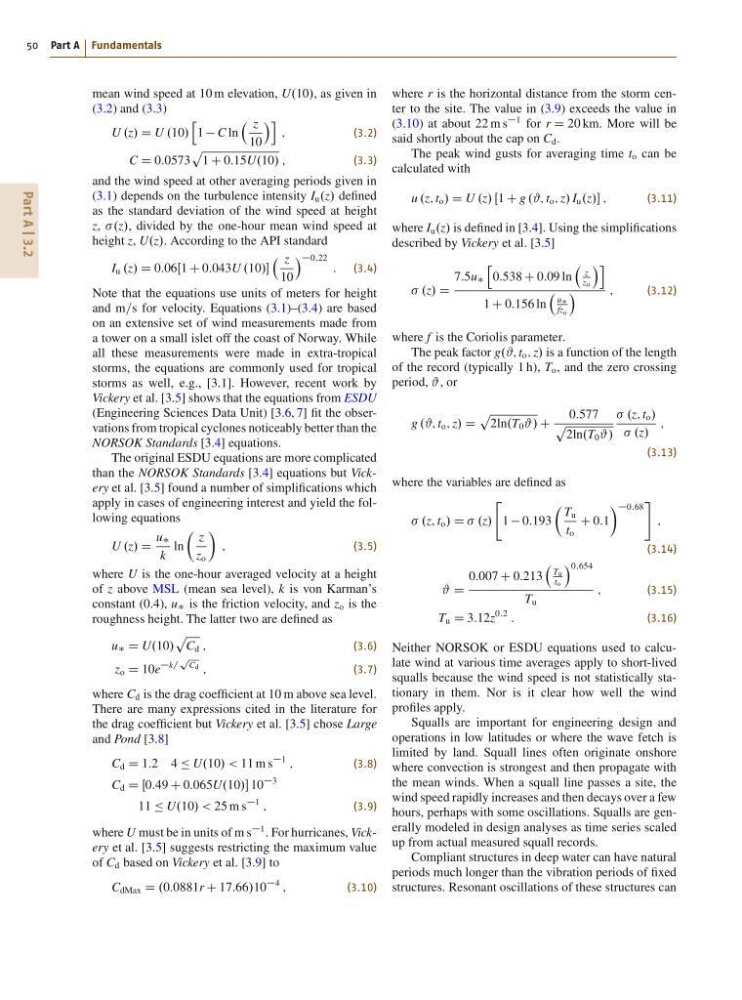
mean wind speed at 10 m elevation, U.10/, as given in
(3.2) and (3.3)
U .z/ D U .10/
h
1 C ln
z
10
Ái
;
(3.2)
C D 0:0573
p
1 C 0:15U.10/ ;
(3.3)
and the wind speed at other averaging periods given in
(3.1) depends on the turbulence intensity I u .z/ defined
as the standard deviation of the wind speed at height
z, .z/, divided by the one-hour mean wind speed at
height z, U.z/. According to the API standard
I u .z/ D 0:06Œ1 C 0:043U .10/
z
10
Á 0:22 : (3.4)
Note that the equations use units of meters for height
and m=s for velocity. Equations (3.1)–(3.4) are based
on an extensive set of wind measurements made from
a tower on a small islet off the coast of Norway. While
all these measurements were made in extra-tropical
storms, the equations are commonly used for tropical
storms as well, e.g., [3.1]. However, recent work by
Vickery et al. [3.5] shows that the equations from ESDU
(Engineering Sciences Data Unit) [3.6, 7] fit the observations from tropical cyclones noticeably better than the
NORSOK Standards [3.4] equations.
The original ESDU equations are more complicated
than the NORSOK Standards [3.4] equations but Vickery et al. [3.5] found a number of simplifications which
apply in cases of engineering interest and yield the following equations
U .z/ D
u
k
ln
 z
z o
Ã
;
(3.5)
where U is the one-hour averaged velocity at a height
of z above MSL (mean sea level), k is von Karman’s
constant (0.4), u is the friction velocity, and z o is the
roughness height. The latter two are defined as
u D U.10/
p
C d ;
(3.6)
z o D 10e
k=
p
Cd
;
(3.7)
where C d is the drag coefficient at 10 m above sea level.
There are many expressions cited in the literature for
the drag coefficient but Vickery et al. [3.5] chose Large
and Pond [3.8]
C d D 1:2 4 Ä U.10/ < 11 m s
1
;
(3.8)
C d D Œ0:49 C 0:065U.10/ 10
3
11 Ä U.10/ < 25 m s
1
;
(3.9)
where U must be in units of m s
1 . For hurricanes, Vickery et al. [3.5] suggests restricting the maximum value
of C d based on Vickery et al. [3.9] to
C dMax D .0:0881r C 17:66/10
4
;
(3.10)
where r is the horizontal distance from the storm center to the site. The value in (3.9) exceeds the value in
(3.10) at about 22 m s
1 for r D 20 km. More will be
said shortly about the cap on C d .
The peak wind gusts for averaging time t o can be
calculated with
u .z; t o / D U .z/ Œ1 C g .#; t o ; z/ I u .z/ ;
(3.11)
where I u .z/ is defined in [3.4]. Using the simplifications
described by Vickery et al. [3.5]
.z/ D
7:5u
h
0:538 C 0:09 ln
z
zo
Ái
1 C 0:156 ln
u
fz o
Á
;
(3.12)
where f is the Coriolis parameter.
The peak factor g.#; t o ; z/ is a function of the length
of the record (typically 1 h), T o , and the zero crossing
period, #, or
g .#; t o ; z/ D
p
2ln.T 0 #/ C
0:577
p
2ln.T 0 #/
.z; t o /
.z/
;
(3.13)
where the variables are defined as
.z; t o / D .z/
"
1 0:193
 T u
t o
C 0:1
à 0:68
#
;
(3.14)
# D
0:007 C 0:213
Tu
to
Á 0:654
T u
;
(3.15)
T u D 3:12z
0:2
:
(3.16)
Neither NORSOK or ESDU equations used to calculate wind at various time averages apply to short-lived
squalls because the wind speed is not statistically stationary in them. Nor is it clear how well the wind
profiles apply.
Squalls are important for engineering design and
operations in low latitudes or where the wave fetch is
limited by land. Squall lines often originate onshore
where convection is strongest and then propagate with
the mean winds. When a squall line passes a site, the
wind speed rapidly increases and then decays over a few
hours, perhaps with some oscillations. Squalls are generally modeled in design analyses as time series scaled
up from actual measured squall records.
Compliant structures in deep water can have natural
periods much longer than the vibration periods of fixed
structures. Resonant oscillations of these structures can
50 Part A Fundamentals
mean wind speed at 10 m elevation, U.10/, as given in
(3.2) and (3.3)
U .z/ D U .10/
h
1 C ln
z
10
Ái
;
(3.2)
C D 0:0573
p
1 C 0:15U.10/ ;
(3.3)
and the wind speed at other averaging periods given in
(3.1) depends on the turbulence intensity I u .z/ defined
as the standard deviation of the wind speed at height
z, .z/, divided by the one-hour mean wind speed at
height z, U.z/. According to the API standard
I u .z/ D 0:06Œ1 C 0:043U .10/
z
10
Á 0:22 : (3.4)
Note that the equations use units of meters for height
and m=s for velocity. Equations (3.1)–(3.4) are based
on an extensive set of wind measurements made from
a tower on a small islet off the coast of Norway. While
all these measurements were made in extra-tropical
storms, the equations are commonly used for tropical
storms as well, e.g., [3.1]. However, recent work by
Vickery et al. [3.5] shows that the equations from ESDU
(Engineering Sciences Data Unit) [3.6, 7] fit the observations from tropical cyclones noticeably better than the
NORSOK Standards [3.4] equations.
The original ESDU equations are more complicated
than the NORSOK Standards [3.4] equations but Vickery et al. [3.5] found a number of simplifications which
apply in cases of engineering interest and yield the following equations
U .z/ D
u
k
ln
 z
z o
Ã
;
(3.5)
where U is the one-hour averaged velocity at a height
of z above MSL (mean sea level), k is von Karman’s
constant (0.4), u is the friction velocity, and z o is the
roughness height. The latter two are defined as
u D U.10/
p
C d ;
(3.6)
z o D 10e
k=
p
Cd
;
(3.7)
where C d is the drag coefficient at 10 m above sea level.
There are many expressions cited in the literature for
the drag coefficient but Vickery et al. [3.5] chose Large
and Pond [3.8]
C d D 1:2 4 Ä U.10/ < 11 m s
1
;
(3.8)
C d D Œ0:49 C 0:065U.10/ 10
3
11 Ä U.10/ < 25 m s
1
;
(3.9)
where U must be in units of m s
1 . For hurricanes, Vickery et al. [3.5] suggests restricting the maximum value
of C d based on Vickery et al. [3.9] to
C dMax D .0:0881r C 17:66/10
4
;
(3.10)
where r is the horizontal distance from the storm center to the site. The value in (3.9) exceeds the value in
(3.10) at about 22 m s
1 for r D 20 km. More will be
said shortly about the cap on C d .
The peak wind gusts for averaging time t o can be
calculated with
u .z; t o / D U .z/ Œ1 C g .#; t o ; z/ I u .z/ ;
(3.11)
where I u .z/ is defined in [3.4]. Using the simplifications
described by Vickery et al. [3.5]
.z/ D
7:5u
h
0:538 C 0:09 ln
z
zo
Ái
1 C 0:156 ln
u
fz o
Á
;
(3.12)
where f is the Coriolis parameter.
The peak factor g.#; t o ; z/ is a function of the length
of the record (typically 1 h), T o , and the zero crossing
period, #, or
g .#; t o ; z/ D
p
2ln.T 0 #/ C
0:577
p
2ln.T 0 #/
.z; t o /
.z/
;
(3.13)
where the variables are defined as
.z; t o / D .z/
"
1 0:193
 T u
t o
C 0:1
à 0:68
#
;
(3.14)
# D
0:007 C 0:213
Tu
to
Á 0:654
T u
;
(3.15)
T u D 3:12z
0:2
:
(3.16)
Neither NORSOK or ESDU equations used to calculate wind at various time averages apply to short-lived
squalls because the wind speed is not statistically stationary in them. Nor is it clear how well the wind
profiles apply.
Squalls are important for engineering design and
operations in low latitudes or where the wave fetch is
limited by land. Squall lines often originate onshore
where convection is strongest and then propagate with
the mean winds. When a squall line passes a site, the
wind speed rapidly increases and then decays over a few
hours, perhaps with some oscillations. Squalls are generally modeled in design analyses as time series scaled
up from actual measured squall records.
Compliant structures in deep water can have natural
periods much longer than the vibration periods of fixed
structures. Resonant oscillations of these structures can