

Autonomy: Risk Assessment 24.2 Risk of Failure 529
Part B | 24.2
9 Work to
reduce A based
on mitigation
plan so A < L
11 Campaign
takes place
5
Demonstrate
that this is so
1
10
Decisions that may
postpone or cancel
the campaign
8
Owner
may increase
L?
No
Yes
7
PI
may reassess
requirements
4
Is
A < L?
Responsible owner
states acceptable probability
of loss (L) for the campaign
2 Principal investigator
sets out campaign
requirements
Yes
3 Technical team assess
probability of loss in light of
this defined campaign (A)
6 Identify key risk factors
Produce mitigation plan
Model effect of mitigation
In
parallel
Reassess
modelled
mitigation
Yes
No
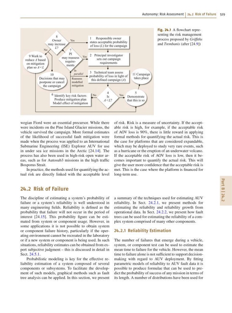
Fig. 24.1 A flowchart representing the risk management
process proposed by Griffiths
and Trembanis (after [24.9])
wegian Fiord were an essential precursor. While there
were incidents on the Pine Island Glacier missions, the
vehicle survived the campaign. More formal estimates
of the likelihood of successful fault mitigation were
made when the process was applied to an International
Submarine Engineering (ISE) Explorer AUV for use
in under sea ice missions in the Arctic [24.14]. The
process has also been used in high-risk open water areas, such as for Autosub3 missions in the high traffic
Bosporus Strait.
In practice, the methods used for quantifying the actual risk are directly linked with the acceptable level
of risk. Risk is a measure of uncertainty. If the acceptable risk is high, for example, if the acceptable risk
of AOV loss is 90%, there is little reward in applying
formal methods for quantifying the actual risk. This is
the case for platforms that are considered expandable,
which may be deployed to study very rare events, such
as a hurricane or the eruption of an underwater volcano.
If the acceptable risk of AOV loss is low, then it becomes important to quantify the actual risk. This will
give the user more confidence that the acceptable risk is
met. This is the case where the platform is financed for
long-term use.
24.2 Risk of Failure
The discipline of estimating a system’s probability of
failure or a system’s reliability is well understood in
many engineering fields. Reliability is defined as the
probability that failure will not occur in the period of
interest [24.15]. This probability figure can be estimated from system or component usage. However, in
some applications it is not possible to obtain system
or component failure history, particularly if the operating environment cannot be recreated in the laboratory
or if a new system or component is being used. In such
situations, reliability estimates can be obtained from expert subjective judgment – this is discussed in detail in
Sect. 24.5.1.
Probabilistic modeling is key for the effective reliability estimation of a system composed of several
components or subsystems. To facilitate the development of such models, graphical methods such as fault
tree analysis can be applied. In this section, we present
a summary of the techniques used for estimating AUV
reliability. In Sect. 24.2.1, we present methods for
estimating the reliability and reliability growth from
operational data. In Sect. 24.2.2, we present how fault
trees can be used for estimating the reliability of a complex system comprised of many other components.
24.2.1 Reliability Estimation
The number of failures that emerge during a vehicle,
system, or component test can be used to estimate the
mean time to failure for the vehicle. However, the mean
time to failure alone is not sufficient to support decisionmaking with regard to AUV deployment. By fitting
parametric models of reliability to AUV fault data it is
possible to produce formulae that can be used to predict the probability of success of any mission in terms of
its length. A number of distributions have been used for
Part B | 24.2
9 Work to
reduce A based
on mitigation
plan so A < L
11 Campaign
takes place
5
Demonstrate
that this is so
1
10
Decisions that may
postpone or cancel
the campaign
8
Owner
may increase
L?
No
Yes
7
PI
may reassess
requirements
4
Is
A < L?
Responsible owner
states acceptable probability
of loss (L) for the campaign
2 Principal investigator
sets out campaign
requirements
Yes
3 Technical team assess
probability of loss in light of
this defined campaign (A)
6 Identify key risk factors
Produce mitigation plan
Model effect of mitigation
In
parallel
Reassess
modelled
mitigation
Yes
No
Fig. 24.1 A flowchart representing the risk management
process proposed by Griffiths
and Trembanis (after [24.9])
wegian Fiord were an essential precursor. While there
were incidents on the Pine Island Glacier missions, the
vehicle survived the campaign. More formal estimates
of the likelihood of successful fault mitigation were
made when the process was applied to an International
Submarine Engineering (ISE) Explorer AUV for use
in under sea ice missions in the Arctic [24.14]. The
process has also been used in high-risk open water areas, such as for Autosub3 missions in the high traffic
Bosporus Strait.
In practice, the methods used for quantifying the actual risk are directly linked with the acceptable level
of risk. Risk is a measure of uncertainty. If the acceptable risk is high, for example, if the acceptable risk
of AOV loss is 90%, there is little reward in applying
formal methods for quantifying the actual risk. This is
the case for platforms that are considered expandable,
which may be deployed to study very rare events, such
as a hurricane or the eruption of an underwater volcano.
If the acceptable risk of AOV loss is low, then it becomes important to quantify the actual risk. This will
give the user more confidence that the acceptable risk is
met. This is the case where the platform is financed for
long-term use.
24.2 Risk of Failure
The discipline of estimating a system’s probability of
failure or a system’s reliability is well understood in
many engineering fields. Reliability is defined as the
probability that failure will not occur in the period of
interest [24.15]. This probability figure can be estimated from system or component usage. However, in
some applications it is not possible to obtain system
or component failure history, particularly if the operating environment cannot be recreated in the laboratory
or if a new system or component is being used. In such
situations, reliability estimates can be obtained from expert subjective judgment – this is discussed in detail in
Sect. 24.5.1.
Probabilistic modeling is key for the effective reliability estimation of a system composed of several
components or subsystems. To facilitate the development of such models, graphical methods such as fault
tree analysis can be applied. In this section, we present
a summary of the techniques used for estimating AUV
reliability. In Sect. 24.2.1, we present methods for
estimating the reliability and reliability growth from
operational data. In Sect. 24.2.2, we present how fault
trees can be used for estimating the reliability of a complex system comprised of many other components.
24.2.1 Reliability Estimation
The number of failures that emerge during a vehicle,
system, or component test can be used to estimate the
mean time to failure for the vehicle. However, the mean
time to failure alone is not sufficient to support decisionmaking with regard to AUV deployment. By fitting
parametric models of reliability to AUV fault data it is
possible to produce formulae that can be used to predict the probability of success of any mission in terms of
its length. A number of distributions have been used for