

Cooperative Vehicle Environmental Monitoring 19.3 Advances in Cooperative Vehicle Ocean Monitoring 449
Part B | 19.3
optimize a sampling performance metric. Second, the
pattern can be chosen for minimal performance sensitivity to disturbances in vehicle motion. Additionally,
the pattern can be chosen to account for design requirements and constraints, such as avoiding or focusing
on certain regions, leveraging information on the direction of strong currents so vehicles move with them
rather than against them, and accommodating additions
or removals of vehicles. Human-in-the-loop supervisory control, which can be critical for highly complex
settings, can be fairly easily integrated when it is warranted. In the ASAP experiment, a team of scientists
made supervisory decisions based on visualizations of
observational data, modeling output, system performance, and availability of vehicles. A method was in
place to translate these decisions into formal adaptations of the desired motion patterns, which could be
refined using numerical optimization tools. To implement an adaptation, an intermittent, discrete change in
the pattern was input to the GCCS and the vehicle network responded accordingly.
The sampling metric used to design motion patterns [19.6] is computed from the mapping error of
the data assimilation scheme known as OA [19.45, 46].
OA provides a linear statistical estimation of a sampled field, and the mapping error measures the residual
uncertainty. OA mapping error is a sampling perfora) Latitude (°)
b) Latitude (°)
–122.8
–122.6
–122.4
Mapping error
–122.2
Longitude (°)
37.3
37.2
37.1
37
36.9
36.8
36.7
1
0.9
0.8
0.7
0.6
0.5
0.4
0.3
0.2
0.1
0
–122.8
–122.6
Point Año Nuevo
1 0 0 0 m
4
0
0
m
1
5
0
m
5
0
m
4 0 k m
2 4
k m
ASAP domain
R
e
la
x
a
ti
o
n
/u
p
w
e
ll
in
g
–122.4
–122.2
Longitude (°)
37.3
37.2
37.1
37
36.9
36.8
36.7
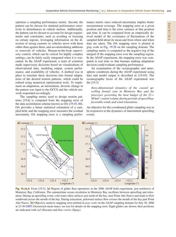
Fig. 19.2a,b From [19.3]. (a) Region of glider fleet operations in the 2006 ASAP field experiment, just northwest of
Monterey Bay, California. The summertime ocean circulation in Monterey Bay oscillates between upwelling and relaxation. During an upwelling event, cold water often surfaces just north of the bay, near Point Año Nuevo and tends to flow
southward across the mouth of the bay. During relaxation, poleward surface flow crosses the mouth of the bay past Point
Año Nuevo. (b) Objective analysis mapping error plotted in gray scale on the ASAP sampling domain for July 30, 2006
at 23:30 GMT (Greenwich mean time); see text for details on the mapping error. Eight gliders are shown; their positions
are indicated with red (Slocum) and blue circles (Spray)
mance metric since reduced uncertainty implies better
measurement coverage. The mapping error at a given
position and time is the error variance at that position
and time. It can be computed from an empirically derived model of the covariance of fluctuations of the
sampled field about its mean and from where and when
data are taken. The OA mapping error is plotted in
gray scale in Fig. 19.2b on the sampling domain. The
sampling metric is computed as the negative log of the
integral of the mapping error over the sampling region.
In the ASAP experiment, the mapping error was computed in real time so that humans making adaptation
decision could evaluate sampling performance.
An examination of the oceanographic and atmospheric conditions during the ASAP experiment using
data and model output is described in [19.93]. The
oceanographic focus of the ASAP experiment was
the [19.3]
three-dimensional dynamics of the coastal upwelling frontal zone in Monterey Bay and the
processes governing the heat budget of the 22
40 km
2 control volume during periods of upwellingfavorable winds and wind relaxations.
An objective for the coordinated glider sampling was to
be responsive to the dynamics of intermittent upwelling
events.
Part B | 19.3
optimize a sampling performance metric. Second, the
pattern can be chosen for minimal performance sensitivity to disturbances in vehicle motion. Additionally,
the pattern can be chosen to account for design requirements and constraints, such as avoiding or focusing
on certain regions, leveraging information on the direction of strong currents so vehicles move with them
rather than against them, and accommodating additions
or removals of vehicles. Human-in-the-loop supervisory control, which can be critical for highly complex
settings, can be fairly easily integrated when it is warranted. In the ASAP experiment, a team of scientists
made supervisory decisions based on visualizations of
observational data, modeling output, system performance, and availability of vehicles. A method was in
place to translate these decisions into formal adaptations of the desired motion patterns, which could be
refined using numerical optimization tools. To implement an adaptation, an intermittent, discrete change in
the pattern was input to the GCCS and the vehicle network responded accordingly.
The sampling metric used to design motion patterns [19.6] is computed from the mapping error of
the data assimilation scheme known as OA [19.45, 46].
OA provides a linear statistical estimation of a sampled field, and the mapping error measures the residual
uncertainty. OA mapping error is a sampling perfora) Latitude (°)
b) Latitude (°)
–122.8
–122.6
–122.4
Mapping error
–122.2
Longitude (°)
37.3
37.2
37.1
37
36.9
36.8
36.7
1
0.9
0.8
0.7
0.6
0.5
0.4
0.3
0.2
0.1
0
–122.8
–122.6
Point Año Nuevo
1 0 0 0 m
4
0
0
m
1
5
0
m
5
0
m
4 0 k m
2 4
k m
ASAP domain
R
e
la
x
a
ti
o
n
/u
p
w
e
ll
in
g
–122.4
–122.2
Longitude (°)
37.3
37.2
37.1
37
36.9
36.8
36.7
Fig. 19.2a,b From [19.3]. (a) Region of glider fleet operations in the 2006 ASAP field experiment, just northwest of
Monterey Bay, California. The summertime ocean circulation in Monterey Bay oscillates between upwelling and relaxation. During an upwelling event, cold water often surfaces just north of the bay, near Point Año Nuevo and tends to flow
southward across the mouth of the bay. During relaxation, poleward surface flow crosses the mouth of the bay past Point
Año Nuevo. (b) Objective analysis mapping error plotted in gray scale on the ASAP sampling domain for July 30, 2006
at 23:30 GMT (Greenwich mean time); see text for details on the mapping error. Eight gliders are shown; their positions
are indicated with red (Slocum) and blue circles (Spray)
mance metric since reduced uncertainty implies better
measurement coverage. The mapping error at a given
position and time is the error variance at that position
and time. It can be computed from an empirically derived model of the covariance of fluctuations of the
sampled field about its mean and from where and when
data are taken. The OA mapping error is plotted in
gray scale in Fig. 19.2b on the sampling domain. The
sampling metric is computed as the negative log of the
integral of the mapping error over the sampling region.
In the ASAP experiment, the mapping error was computed in real time so that humans making adaptation
decision could evaluate sampling performance.
An examination of the oceanographic and atmospheric conditions during the ASAP experiment using
data and model output is described in [19.93]. The
oceanographic focus of the ASAP experiment was
the [19.3]
three-dimensional dynamics of the coastal upwelling frontal zone in Monterey Bay and the
processes governing the heat budget of the 22
40 km
2 control volume during periods of upwellingfavorable winds and wind relaxations.
An objective for the coordinated glider sampling was to
be responsive to the dynamics of intermittent upwelling
events.