

Part B | 15.4
370 Part B Autonomous Ocean Vehicles, Subsystems and Control
Δf
...
B = KΔ f
f
f k → f k (1+ a)
f
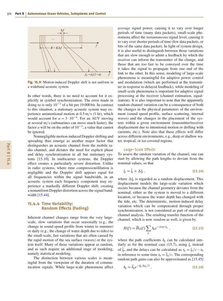
Fig. 15.11 Motion-induced Doppler shift is not uniform in
a wideband acoustic system
In other words, there is no need to account for it explicitly in symbol synchronization. The error made in
doing so is only 10
3 of a bit per 10 000 bit. In contrast
to this situation, a stationary acoustic system may experience unintentional motion at 0:5 m=s (1 kt), which
would account for a D 3 10
4 . For an AUV moving
at several m=s (submarines can move much faster), the
factor a will be on the order of 10
3 , a value that cannot
be ignored.
Nonnegligible motion-induced Doppler shifting and
spreading thus emerge as another major factor that
distinguishes an acoustic channel from the mobile radio channel, and dictates the need for explicit phase
and delay synchronization in all but stationary systems [15.10]. In multicarrier systems, the Doppler
effect creates a particularly severe distortion. Unlike
in radio systems, where time compression/dilation is
negligible and the Doppler shift appears equal for
all frequencies within the signal bandwidth, in an
acoustic system each frequency component may experience a markedly different Doppler shift, creating
a nonuniform Doppler distortion across the signal bandwidth [15.44].
15.4.4 Time Variability:
Random Effects (Fading)
Inherent channel changes range from the very largescale, slow variations that occur seasonally (e.g., the
change in sound speed profile from winter to summer)
or daily (e.g., the change of water depth due to tides) to
the small-scale, fast variations that are often caused by
the rapid motion of the sea surface (waves) or the system itself. Many of these variations appear as random,
and as such require an additional stage of modeling,
namely statistical modeling.
The distinction between various scales is meaningful from the viewpoint of the duration of communication signals. While large-scale phenomena affect
average signal power, causing it to vary over longer
periods of time (many data packets), small-scale phenomena affect the instantaneous signal level, causing it
to vary over shorter periods of time (few data packets, or
bits of the same data packet). In light of system design,
it is also useful to distinguish between those variations
that are slow enough to admit a feedback by which the
receiver can inform the transmitter of the change, and
those that are too fast to be conveyed over the time
it takes the signal to propagate from one end of the
link to the other. In this sense, modeling of large-scale
phenomena is meaningful for adaptive power control
and modulation (which are performed at the transmitter in response to delayed feedback), while modeling of
small-scale phenomena is important for adaptive signal
processing at the receiver (channel estimation, equalization). It is also important to note that the apparently
random channel variation can be a consequence of both
the changes in the physical parameters of the environment (sound speed profile, surface scattering, internal
waves) and the changes in the placement of the system within a given environment (transmitter/receiver
displacement due to intentional motion or drifting with
currents, etc.). Note also that these effects will differ
across different environments, e.g., deep or shallow water, tropical, or ice-covered regions.
Large-Scale Effects
To assess the random variation of the channel, one can
start by allowing the path lengths to deviate from the
nominal values, so that
l p D l p C l p ;
(15.14)
where l p is regarded as a random displacement. This
displacement models the large-scale variation which
occurs because the channel geometry deviates from the
nominal, either as the system is moved to a different
location, or because the water depth has changed with
the tide, etc. The deterministic, motion-induced delay
variation which can be compensated through proper
synchronization, is not considered as part of statistical
channel analysis. The resulting transfer function of the
channel, which is now random as well, is given by
H.f / D H 0 .f /
X
p
h p e
i2f p
;
(15.15)
where the path coefficients h p can be calculated similarly as for the nominal case (15.7), using l p instead
of l p , and the delays can be calculated as p D l p =c t 0
in reference to some time t 0 D l 0 =c. The corresponding
random path gains can also be approximated as [15.45]
h p D h p e
plp=2
;
(15.16)
370 Part B Autonomous Ocean Vehicles, Subsystems and Control
Δf
...
B = KΔ f
f
f k → f k (1+ a)
f
Fig. 15.11 Motion-induced Doppler shift is not uniform in
a wideband acoustic system
In other words, there is no need to account for it explicitly in symbol synchronization. The error made in
doing so is only 10
3 of a bit per 10 000 bit. In contrast
to this situation, a stationary acoustic system may experience unintentional motion at 0:5 m=s (1 kt), which
would account for a D 3 10
4 . For an AUV moving
at several m=s (submarines can move much faster), the
factor a will be on the order of 10
3 , a value that cannot
be ignored.
Nonnegligible motion-induced Doppler shifting and
spreading thus emerge as another major factor that
distinguishes an acoustic channel from the mobile radio channel, and dictates the need for explicit phase
and delay synchronization in all but stationary systems [15.10]. In multicarrier systems, the Doppler
effect creates a particularly severe distortion. Unlike
in radio systems, where time compression/dilation is
negligible and the Doppler shift appears equal for
all frequencies within the signal bandwidth, in an
acoustic system each frequency component may experience a markedly different Doppler shift, creating
a nonuniform Doppler distortion across the signal bandwidth [15.44].
15.4.4 Time Variability:
Random Effects (Fading)
Inherent channel changes range from the very largescale, slow variations that occur seasonally (e.g., the
change in sound speed profile from winter to summer)
or daily (e.g., the change of water depth due to tides) to
the small-scale, fast variations that are often caused by
the rapid motion of the sea surface (waves) or the system itself. Many of these variations appear as random,
and as such require an additional stage of modeling,
namely statistical modeling.
The distinction between various scales is meaningful from the viewpoint of the duration of communication signals. While large-scale phenomena affect
average signal power, causing it to vary over longer
periods of time (many data packets), small-scale phenomena affect the instantaneous signal level, causing it
to vary over shorter periods of time (few data packets, or
bits of the same data packet). In light of system design,
it is also useful to distinguish between those variations
that are slow enough to admit a feedback by which the
receiver can inform the transmitter of the change, and
those that are too fast to be conveyed over the time
it takes the signal to propagate from one end of the
link to the other. In this sense, modeling of large-scale
phenomena is meaningful for adaptive power control
and modulation (which are performed at the transmitter in response to delayed feedback), while modeling of
small-scale phenomena is important for adaptive signal
processing at the receiver (channel estimation, equalization). It is also important to note that the apparently
random channel variation can be a consequence of both
the changes in the physical parameters of the environment (sound speed profile, surface scattering, internal
waves) and the changes in the placement of the system within a given environment (transmitter/receiver
displacement due to intentional motion or drifting with
currents, etc.). Note also that these effects will differ
across different environments, e.g., deep or shallow water, tropical, or ice-covered regions.
Large-Scale Effects
To assess the random variation of the channel, one can
start by allowing the path lengths to deviate from the
nominal values, so that
l p D l p C l p ;
(15.14)
where l p is regarded as a random displacement. This
displacement models the large-scale variation which
occurs because the channel geometry deviates from the
nominal, either as the system is moved to a different
location, or because the water depth has changed with
the tide, etc. The deterministic, motion-induced delay
variation which can be compensated through proper
synchronization, is not considered as part of statistical
channel analysis. The resulting transfer function of the
channel, which is now random as well, is given by
H.f / D H 0 .f /
X
p
h p e
i2f p
;
(15.15)
where the path coefficients h p can be calculated similarly as for the nominal case (15.7), using l p instead
of l p , and the delays can be calculated as p D l p =c t 0
in reference to some time t 0 D l 0 =c. The corresponding
random path gains can also be approximated as [15.45]
h p D h p e
plp=2
;
(15.16)