

Part B | 14.2
348 Part B Autonomous Ocean Vehicles, Subsystems and Control
with
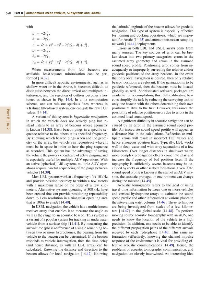
a 1 D D2x
0
2 ;
b 1 D D2y
0
2 ;
c 1 D x
02
2 C y
02
2 C z
02
2 2z
0 z
0
2 d
2
2 C d
2
1 ;
a 2 D D2x
0
3 ;
b 2 D D2y
0
3 ;
c 2 D x
02
3 C y
02
3 C z
02
3 2z
0 z
0
3 d
2
3 C d
2
1 :
When measurements from four beacons are
available, least-squares minimization can be performed [14.37].
In more difficult acoustic environments, such as in
shallow water or in the Arctic, it becomes difficult to
distinguish between the direct arrival and multipath interference, and the rejection of outliers becomes a key
issue, as shown in Fig. 14.4. In a fix computation
scheme, one can rule out spurious fixes, whereas in
a Kalman filter-based system, one can gate the raw TOF
values [14.14].
A variant of this system is hyperbolic navigation,
in which the vehicle does not actively ping but instead listens to an array of beacons whose geometry
is known [14.38]. Each beacon pings in a specific sequence relative to the others at its specified frequency.
By knowing which beacon pings when and the geometry of the array, the vehicle can reconstruct where it
must be in space in order to hear the ping sequence
as recorded. This system has the advantage of saving
the vehicle the power expenditure of active pinging, and
is especially useful for multiple AUV operations. With
an active (spherical) LBL system, multiple AUV operations require careful sequencing of the pings between
vehicles [14.39].
Most LBL systems work at a frequency of 10 kHz
and provide position accuracy to within a few meters
with a maximum range of the order of a few kilometers. Alternative systems operating at 300 kHz have
been created that can provide positioning repeatability
down to 1 cm resolution in a triangular operating area
that is 100 m to a side [14.40].
In USBL navigation, the vehicle has a multielement
receiver array that enables it to measure the angle as
well as the range to an acoustic beacon. This system is
a variant of a popular system for tracking an underwater
vehicle from a surface ship [14.41]. By measuring the
arrival time (phase) difference of a single sonar ping between two or more hydrophones, the bearing from the
vehicle to the beacon can be determined. If the beacon
responds to vehicle interrogation, then the time delay
(and hence distance, as with an LBL array) can be
calculated. Knowing the distance and direction to the
beacon allows for local navigation [14.42]. Knowing
the latitude/longitude of the beacon allows for geodetic
navigation. This type of system is especially effective
for homing and docking operations, which are important for Arctic [14.43] and autonomous ocean sampling
network [14.44] deployments.
Errors in both LBL and USBL arrays come from
many sources. The key sources of error can be broken down into two primary categories: errors in the
assumed array geometry and errors in the assumed
sound speed profile. Positioning error comes from inadequately or improperly surveying the relative and/or
geodetic positions of the array beacons. In the event
that only local navigation is desired, then only relative
beacon positions are relevant. If the navigation is to be
geodetic-referenced, then the beacons must be located
globally as well. Sophisticated software packages are
available for accomplishing this. Self-calibrating beacons simplify the task by reducing the surveying task to
only one beacon with the others determining their own
positions relative to the first. However, this raises the
possibility of relative position errors due to errors in the
assumed local sound speed.
A significant difficulty in acoustic navigation can be
caused by an error in the assumed sound speed profile. An inaccurate sound speed profile will appear as
a distance bias in the calculations. Reflection or multipath errors will result in incorrect TOF values and
hence erroneous position fixes. Typically, LBL works
well in deep water and with array separations of a few
kilometers. Over longer distances in shallower water,
more complex propagation effects come into play and
increase the frequency of bad position fixes. If the
topography is sufficiently severe, beacons may be occluded by rocks or other seabed formations. Even if the
sound speed profile is known at the start of an AUV mission, the acoustic propagation environment can change
during the mission [14.45].
Acoustic tomography refers to the goal of using
travel time information between one or more vehicles
and vertical hydrophone arrays to estimate the sound
speed profile and other information at various places in
the intervening water column [14.46]. These techniques
are being investigated from scales of a few kilometers [14.47] to the global scale [14.48]. To perform
moving source acoustic tomography with an AUV, one
needs to know the location of the vehicle to a high
precision. In addition, one needs to be able to identify
the different propagation paths of the different arrivals
received by each hydrophone [14.46]. This same information (effectively, knowing the channel impulse
response of the environment) is vital for providing effective acoustic communications [14.49]. Hence, the
problems of acoustic tomography, communication, and
navigation are closely intertwined. An interesting idea
348 Part B Autonomous Ocean Vehicles, Subsystems and Control
with
a 1 D D2x
0
2 ;
b 1 D D2y
0
2 ;
c 1 D x
02
2 C y
02
2 C z
02
2 2z
0 z
0
2 d
2
2 C d
2
1 ;
a 2 D D2x
0
3 ;
b 2 D D2y
0
3 ;
c 2 D x
02
3 C y
02
3 C z
02
3 2z
0 z
0
3 d
2
3 C d
2
1 :
When measurements from four beacons are
available, least-squares minimization can be performed [14.37].
In more difficult acoustic environments, such as in
shallow water or in the Arctic, it becomes difficult to
distinguish between the direct arrival and multipath interference, and the rejection of outliers becomes a key
issue, as shown in Fig. 14.4. In a fix computation
scheme, one can rule out spurious fixes, whereas in
a Kalman filter-based system, one can gate the raw TOF
values [14.14].
A variant of this system is hyperbolic navigation,
in which the vehicle does not actively ping but instead listens to an array of beacons whose geometry
is known [14.38]. Each beacon pings in a specific sequence relative to the others at its specified frequency.
By knowing which beacon pings when and the geometry of the array, the vehicle can reconstruct where it
must be in space in order to hear the ping sequence
as recorded. This system has the advantage of saving
the vehicle the power expenditure of active pinging, and
is especially useful for multiple AUV operations. With
an active (spherical) LBL system, multiple AUV operations require careful sequencing of the pings between
vehicles [14.39].
Most LBL systems work at a frequency of 10 kHz
and provide position accuracy to within a few meters
with a maximum range of the order of a few kilometers. Alternative systems operating at 300 kHz have
been created that can provide positioning repeatability
down to 1 cm resolution in a triangular operating area
that is 100 m to a side [14.40].
In USBL navigation, the vehicle has a multielement
receiver array that enables it to measure the angle as
well as the range to an acoustic beacon. This system is
a variant of a popular system for tracking an underwater
vehicle from a surface ship [14.41]. By measuring the
arrival time (phase) difference of a single sonar ping between two or more hydrophones, the bearing from the
vehicle to the beacon can be determined. If the beacon
responds to vehicle interrogation, then the time delay
(and hence distance, as with an LBL array) can be
calculated. Knowing the distance and direction to the
beacon allows for local navigation [14.42]. Knowing
the latitude/longitude of the beacon allows for geodetic
navigation. This type of system is especially effective
for homing and docking operations, which are important for Arctic [14.43] and autonomous ocean sampling
network [14.44] deployments.
Errors in both LBL and USBL arrays come from
many sources. The key sources of error can be broken down into two primary categories: errors in the
assumed array geometry and errors in the assumed
sound speed profile. Positioning error comes from inadequately or improperly surveying the relative and/or
geodetic positions of the array beacons. In the event
that only local navigation is desired, then only relative
beacon positions are relevant. If the navigation is to be
geodetic-referenced, then the beacons must be located
globally as well. Sophisticated software packages are
available for accomplishing this. Self-calibrating beacons simplify the task by reducing the surveying task to
only one beacon with the others determining their own
positions relative to the first. However, this raises the
possibility of relative position errors due to errors in the
assumed local sound speed.
A significant difficulty in acoustic navigation can be
caused by an error in the assumed sound speed profile. An inaccurate sound speed profile will appear as
a distance bias in the calculations. Reflection or multipath errors will result in incorrect TOF values and
hence erroneous position fixes. Typically, LBL works
well in deep water and with array separations of a few
kilometers. Over longer distances in shallower water,
more complex propagation effects come into play and
increase the frequency of bad position fixes. If the
topography is sufficiently severe, beacons may be occluded by rocks or other seabed formations. Even if the
sound speed profile is known at the start of an AUV mission, the acoustic propagation environment can change
during the mission [14.45].
Acoustic tomography refers to the goal of using
travel time information between one or more vehicles
and vertical hydrophone arrays to estimate the sound
speed profile and other information at various places in
the intervening water column [14.46]. These techniques
are being investigated from scales of a few kilometers [14.47] to the global scale [14.48]. To perform
moving source acoustic tomography with an AUV, one
needs to know the location of the vehicle to a high
precision. In addition, one needs to be able to identify
the different propagation paths of the different arrivals
received by each hydrophone [14.46]. This same information (effectively, knowing the channel impulse
response of the environment) is vital for providing effective acoustic communications [14.49]. Hence, the
problems of acoustic tomography, communication, and
navigation are closely intertwined. An interesting idea