

Digital Signal Processing 9.3 The Fast Fourier Transform (FFT) 215
Part A | 9.3
x (0)
X (0)
x (1)
X (4)
W 8
0
Stage 1
Bit reversed
outputs
–1
x (2)
X (2)
x (3)
X (6)
W 8
0
W 8
2
W 8
0
–1
–1
–1
x (4)
X (1)
x (5)
X (5)
W 8
0
W 8
1
–1
–1
–1
W 8
0
–1
x (6)
X (3)
x (7)
X (7)
W 8
0
W 8
2
W 8
0
W 8
3
W 8
2
–1
–1
–1
–1
–1
Stage 3
Stage 2
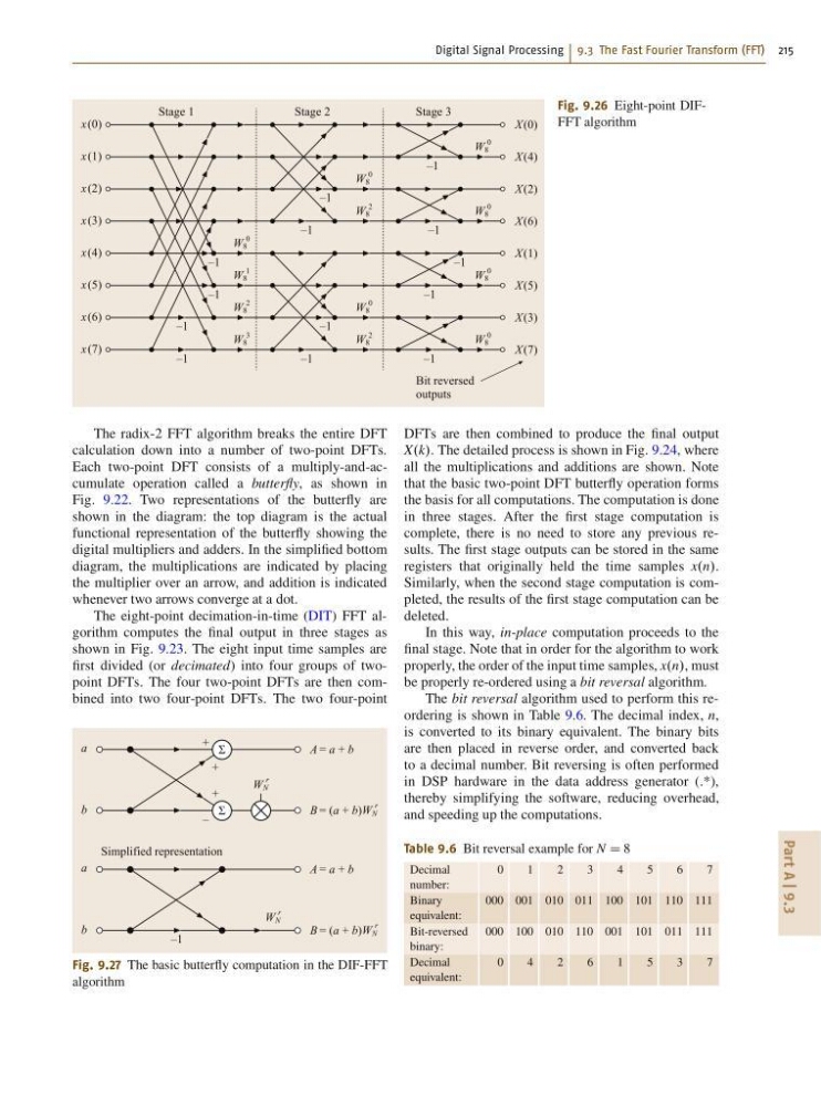
Fig. 9.26 Eight-point DIFFFT algorithm
The radix-2 FFT algorithm breaks the entire DFT
calculation down into a number of two-point DFTs.
Each two-point DFT consists of a multiply-and-accumulate operation called a butterfly, as shown in
Fig. 9.22. Two representations of the butterfly are
shown in the diagram: the top diagram is the actual
functional representation of the butterfly showing the
digital multipliers and adders. In the simplified bottom
diagram, the multiplications are indicated by placing
the multiplier over an arrow, and addition is indicated
whenever two arrows converge at a dot.
The eight-point decimation-in-time (DIT) FFT algorithm computes the final output in three stages as
shown in Fig. 9.23. The eight input time samples are
first divided (or decimated) into four groups of twopoint DFTs. The four two-point DFTs are then combined into two four-point DFTs. The two four-point
a
A = a + b
+
+
+
Σ
b
B = (a + b)W N
r
–
–1
Σ
W N
r
a
Simplified representation
A = a + b
b
B = (a + b)W N
r
W N
r
Fig. 9.27 The basic butterfly computation in the DIF-FFT
algorithm
DFTs are then combined to produce the final output
X.k/. The detailed process is shown in Fig. 9.24, where
all the multiplications and additions are shown. Note
that the basic two-point DFT butterfly operation forms
the basis for all computations. The computation is done
in three stages. After the first stage computation is
complete, there is no need to store any previous results. The first stage outputs can be stored in the same
registers that originally held the time samples x.n/.
Similarly, when the second stage computation is completed, the results of the first stage computation can be
deleted.
In this way, in-place computation proceeds to the
final stage. Note that in order for the algorithm to work
properly, the order of the input time samples, x.n/, must
be properly re-ordered using a bit reversal algorithm.
The bit reversal algorithm used to perform this reordering is shown in Table 9.6. The decimal index, n,
is converted to its binary equivalent. The binary bits
are then placed in reverse order, and converted back
to a decimal number. Bit reversing is often performed
in DSP hardware in the data address generator (.*),
thereby simplifying the software, reducing overhead,
and speeding up the computations.
Table 9.6 Bit reversal example for N D 8
Decimal
number:
0
1
2
3
4
5
6
7
Binary
equivalent:
000 001 010 011 100 101 110 111
Bit-reversed
binary:
000 100 010 110 001 101 011 111
Decimal
equivalent:
0
4
2
6
1
5
3
7
Part A | 9.3
x (0)
X (0)
x (1)
X (4)
W 8
0
Stage 1
Bit reversed
outputs
–1
x (2)
X (2)
x (3)
X (6)
W 8
0
W 8
2
W 8
0
–1
–1
–1
x (4)
X (1)
x (5)
X (5)
W 8
0
W 8
1
–1
–1
–1
W 8
0
–1
x (6)
X (3)
x (7)
X (7)
W 8
0
W 8
2
W 8
0
W 8
3
W 8
2
–1
–1
–1
–1
–1
Stage 3
Stage 2
Fig. 9.26 Eight-point DIFFFT algorithm
The radix-2 FFT algorithm breaks the entire DFT
calculation down into a number of two-point DFTs.
Each two-point DFT consists of a multiply-and-accumulate operation called a butterfly, as shown in
Fig. 9.22. Two representations of the butterfly are
shown in the diagram: the top diagram is the actual
functional representation of the butterfly showing the
digital multipliers and adders. In the simplified bottom
diagram, the multiplications are indicated by placing
the multiplier over an arrow, and addition is indicated
whenever two arrows converge at a dot.
The eight-point decimation-in-time (DIT) FFT algorithm computes the final output in three stages as
shown in Fig. 9.23. The eight input time samples are
first divided (or decimated) into four groups of twopoint DFTs. The four two-point DFTs are then combined into two four-point DFTs. The two four-point
a
A = a + b
+
+
+
Σ
b
B = (a + b)W N
r
–
–1
Σ
W N
r
a
Simplified representation
A = a + b
b
B = (a + b)W N
r
W N
r
Fig. 9.27 The basic butterfly computation in the DIF-FFT
algorithm
DFTs are then combined to produce the final output
X.k/. The detailed process is shown in Fig. 9.24, where
all the multiplications and additions are shown. Note
that the basic two-point DFT butterfly operation forms
the basis for all computations. The computation is done
in three stages. After the first stage computation is
complete, there is no need to store any previous results. The first stage outputs can be stored in the same
registers that originally held the time samples x.n/.
Similarly, when the second stage computation is completed, the results of the first stage computation can be
deleted.
In this way, in-place computation proceeds to the
final stage. Note that in order for the algorithm to work
properly, the order of the input time samples, x.n/, must
be properly re-ordered using a bit reversal algorithm.
The bit reversal algorithm used to perform this reordering is shown in Table 9.6. The decimal index, n,
is converted to its binary equivalent. The binary bits
are then placed in reverse order, and converted back
to a decimal number. Bit reversing is often performed
in DSP hardware in the data address generator (.*),
thereby simplifying the software, reducing overhead,
and speeding up the computations.
Table 9.6 Bit reversal example for N D 8
Decimal
number:
0
1
2
3
4
5
6
7
Binary
equivalent:
000 001 010 011 100 101 110 111
Bit-reversed
binary:
000 100 010 110 001 101 011 111
Decimal
equivalent:
0
4
2
6
1
5
3
7