

Digital Signal Processing 9.1 Discrete-Time Systems 203
Part A | 9.1
tems (LTI) [9.1, 2, 4–6]. Such systems are described in
continuous time by linear differential equations with
constant coefficients. In discrete time, such a differential equation is converted to a difference equation
corresponding to a discrete-time system described by
a transfer function in variable z, or equivalently z
1 .
The general form of a linear difference equation with
input u.n/ and output y.n/ is the following,
y.n/ D
M
X
kD0
b k u.n k/
N
X
kD1
a k y.n k/ :
(9.31)
To obtain the iterative process started in order to obtain
samples of discrete-time output signal y.n/ for n 0, N
initial conditions are needed: y.k/, k D 1; : : : ; N. Using (9.31) we can conclude that the n-th sample of the
output is determined as a weighed sum of the current
plus M past input samples and N past output samples.
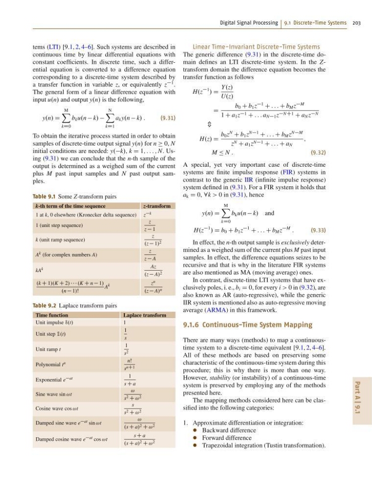
Table 9.1 Some Z-transform pairs
k-th term of the time sequence
z-transform
1 at k, 0 elsewhere (Kronecker delta sequence) z k
1 (unit step sequence)
z
z 1
k (unit ramp sequence)
z
.z 1/ 2
A k (for complex numbers A)
z
z A
kA
k
Az
.z A/ 2
.k C 1/.K C 2/ .K C n 1/
.n 1/Š
A
k
z n
.z A/ n
Table 9.2 Laplace transform pairs
Time function
Laplace transform
Unit impulse •.t/
1
Unit step 1.t/
1
s
Unit ramp t
1
s 2
Polynomial t n
nŠ
s nC1
Exponential e at
1
s C a
Sine wave sin !t
!
s 2 C ! 2
Cosine wave cos !t
s
s 2 C ! 2
Damped sine wave e at sin !t
!
.s C a/ 2 C ! 2
Damped cosine wave e at cos !t
s C a
.s C a/ 2 C ! 2
Linear Time-Invariant Discrete-Time Systems
The generic difference (9.31) in the discrete-time domain defines an LTI discrete-time system. In the Ztransform domain the difference equation becomes the
transfer function as follows
H.z
1
/ D
Y.z/
U.z/
D
b 0 C b 1 z
1
C : : : C b M z
M
1 C a 1 z 1 C : : : a N1 z NC1 C a N z N
m
H.z/ D
b 0 z
N
C b 1 z
N1
C : : : C b M z
NM
z N C a 1 z N1 C : : : C a N
;
M Ä N :
(9.32)
A special, yet very important case of discrete-time
systems are finite impulse response (FIR) systems in
contrast to the generic IIR (infinite impulse response)
system defined in (9.31). For a FIR system it holds that
a k D 0, 8k > 0 in (9.31), hence
y.n/ D
M
X
kD0
b k u.n k/ and
H.z
1
/ D b 0 C b 1 z
1
C : : : C b M z
M
:
(9.33)
In effect, the n-th output sample is exclusively determined as a weighed sum of the current plus M past input
samples. In effect, the difference equations seizes to be
recursive and that is why in the literature FIR systems
are also mentioned as MA (moving average) ones.
In contrast, discrete-time LTI systems that have exclusively poles, i. e., b i D 0, for every i > 0 in (9.32), are
also known as AR (auto-regressive), while the generic
IIR system is mentioned also as auto-regressive moving
average (ARMA) in this framework.
9.1.6 Continuous-Time System Mapping
There are many ways (methods) to map a continuoustime system to a discrete-time equivalent [9.1, 2, 4–6].
All of these methods are based on preserving some
characteristic of the continuous-time system during this
procedure; this is why there is more than one way.
However, stability (or instability) of a continuous-time
system is preserved by employing any of the methods
presented here.
The mapping methods considered here can be classified into the following categories:
1. Approximate differentiation or integration:
Backward difference
Forward difference
Trapezoidal integration (Tustin transformation).
Part A | 9.1
tems (LTI) [9.1, 2, 4–6]. Such systems are described in
continuous time by linear differential equations with
constant coefficients. In discrete time, such a differential equation is converted to a difference equation
corresponding to a discrete-time system described by
a transfer function in variable z, or equivalently z
1 .
The general form of a linear difference equation with
input u.n/ and output y.n/ is the following,
y.n/ D
M
X
kD0
b k u.n k/
N
X
kD1
a k y.n k/ :
(9.31)
To obtain the iterative process started in order to obtain
samples of discrete-time output signal y.n/ for n 0, N
initial conditions are needed: y.k/, k D 1; : : : ; N. Using (9.31) we can conclude that the n-th sample of the
output is determined as a weighed sum of the current
plus M past input samples and N past output samples.
Table 9.1 Some Z-transform pairs
k-th term of the time sequence
z-transform
1 at k, 0 elsewhere (Kronecker delta sequence) z k
1 (unit step sequence)
z
z 1
k (unit ramp sequence)
z
.z 1/ 2
A k (for complex numbers A)
z
z A
kA
k
Az
.z A/ 2
.k C 1/.K C 2/ .K C n 1/
.n 1/Š
A
k
z n
.z A/ n
Table 9.2 Laplace transform pairs
Time function
Laplace transform
Unit impulse •.t/
1
Unit step 1.t/
1
s
Unit ramp t
1
s 2
Polynomial t n
nŠ
s nC1
Exponential e at
1
s C a
Sine wave sin !t
!
s 2 C ! 2
Cosine wave cos !t
s
s 2 C ! 2
Damped sine wave e at sin !t
!
.s C a/ 2 C ! 2
Damped cosine wave e at cos !t
s C a
.s C a/ 2 C ! 2
Linear Time-Invariant Discrete-Time Systems
The generic difference (9.31) in the discrete-time domain defines an LTI discrete-time system. In the Ztransform domain the difference equation becomes the
transfer function as follows
H.z
1
/ D
Y.z/
U.z/
D
b 0 C b 1 z
1
C : : : C b M z
M
1 C a 1 z 1 C : : : a N1 z NC1 C a N z N
m
H.z/ D
b 0 z
N
C b 1 z
N1
C : : : C b M z
NM
z N C a 1 z N1 C : : : C a N
;
M Ä N :
(9.32)
A special, yet very important case of discrete-time
systems are finite impulse response (FIR) systems in
contrast to the generic IIR (infinite impulse response)
system defined in (9.31). For a FIR system it holds that
a k D 0, 8k > 0 in (9.31), hence
y.n/ D
M
X
kD0
b k u.n k/ and
H.z
1
/ D b 0 C b 1 z
1
C : : : C b M z
M
:
(9.33)
In effect, the n-th output sample is exclusively determined as a weighed sum of the current plus M past input
samples. In effect, the difference equations seizes to be
recursive and that is why in the literature FIR systems
are also mentioned as MA (moving average) ones.
In contrast, discrete-time LTI systems that have exclusively poles, i. e., b i D 0, for every i > 0 in (9.32), are
also known as AR (auto-regressive), while the generic
IIR system is mentioned also as auto-regressive moving
average (ARMA) in this framework.
9.1.6 Continuous-Time System Mapping
There are many ways (methods) to map a continuoustime system to a discrete-time equivalent [9.1, 2, 4–6].
All of these methods are based on preserving some
characteristic of the continuous-time system during this
procedure; this is why there is more than one way.
However, stability (or instability) of a continuous-time
system is preserved by employing any of the methods
presented here.
The mapping methods considered here can be classified into the following categories:
1. Approximate differentiation or integration:
Backward difference
Forward difference
Trapezoidal integration (Tustin transformation).