

Part A | 7.1
136 Part A Fundamentals
Threedimensional
vortex
breakdown
Spanwise
vorticity
Turbulent
spots
Edge
contamination
Transition length
Laminar
Turbulent
Re crit
x
U
U
0
δ (x)
Fully
turbulent
flow
Stable
laminar
flow
T/S
waves
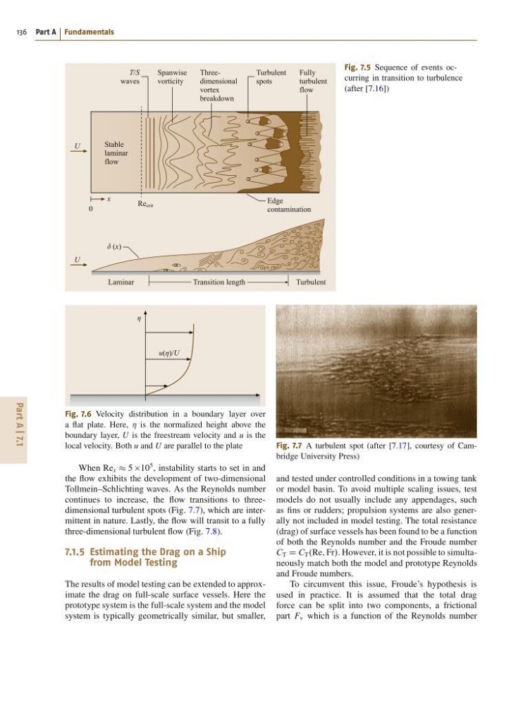
Fig. 7.5 Sequence of events occurring in transition to turbulence
(after [7.16])
u(η)/U
η
Fig. 7.6 Velocity distribution in a boundary layer over
a flat plate. Here, Á is the normalized height above the
boundary layer, U is the freestream velocity and u is the
local velocity. Both u and U are parallel to the plate
When Re x 5 10
5 , instability starts to set in and
the flow exhibits the development of two-dimensional
Tollmein–Schlichting waves. As the Reynolds number
continues to increase, the flow transitions to threedimensional turbulent spots (Fig. 7.7), which are intermittent in nature. Lastly, the flow will transit to a fully
three-dimensional turbulent flow (Fig. 7.8).
7.1.5 Estimating the Drag on a Ship
from Model Testing
The results of model testing can be extended to approximate the drag on full-scale surface vessels. Here the
prototype system is the full-scale system and the model
system is typically geometrically similar, but smaller,
Fig. 7.7 A turbulent spot (after [7.17], courtesy of Cambridge University Press)
and tested under controlled conditions in a towing tank
or model basin. To avoid multiple scaling issues, test
models do not usually include any appendages, such
as fins or rudders; propulsion systems are also generally not included in model testing. The total resistance
(drag) of surface vessels has been found to be a function
of both the Reynolds number and the Froude number
C T D C T .Re; Fr/. However, it is not possible to simultaneously match both the model and prototype Reynolds
and Froude numbers.
To circumvent this issue, Froude’s hypothesis is
used in practice. It is assumed that the total drag
force can be split into two components, a frictional
part F v which is a function of the Reynolds number
136 Part A Fundamentals
Threedimensional
vortex
breakdown
Spanwise
vorticity
Turbulent
spots
Edge
contamination
Transition length
Laminar
Turbulent
Re crit
x
U
U
0
δ (x)
Fully
turbulent
flow
Stable
laminar
flow
T/S
waves
Fig. 7.5 Sequence of events occurring in transition to turbulence
(after [7.16])
u(η)/U
η
Fig. 7.6 Velocity distribution in a boundary layer over
a flat plate. Here, Á is the normalized height above the
boundary layer, U is the freestream velocity and u is the
local velocity. Both u and U are parallel to the plate
When Re x 5 10
5 , instability starts to set in and
the flow exhibits the development of two-dimensional
Tollmein–Schlichting waves. As the Reynolds number
continues to increase, the flow transitions to threedimensional turbulent spots (Fig. 7.7), which are intermittent in nature. Lastly, the flow will transit to a fully
three-dimensional turbulent flow (Fig. 7.8).
7.1.5 Estimating the Drag on a Ship
from Model Testing
The results of model testing can be extended to approximate the drag on full-scale surface vessels. Here the
prototype system is the full-scale system and the model
system is typically geometrically similar, but smaller,
Fig. 7.7 A turbulent spot (after [7.17], courtesy of Cambridge University Press)
and tested under controlled conditions in a towing tank
or model basin. To avoid multiple scaling issues, test
models do not usually include any appendages, such
as fins or rudders; propulsion systems are also generally not included in model testing. The total resistance
(drag) of surface vessels has been found to be a function
of both the Reynolds number and the Froude number
C T D C T .Re; Fr/. However, it is not possible to simultaneously match both the model and prototype Reynolds
and Froude numbers.
To circumvent this issue, Froude’s hypothesis is
used in practice. It is assumed that the total drag
force can be split into two components, a frictional
part F v which is a function of the Reynolds number