

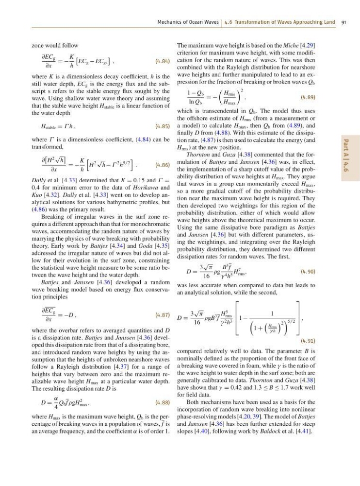
Mechanics of Ocean Waves 4.6 Transformation of Waves Approaching Land 91
Part A | 4.6
zone would follow
@EC g
@x
D D
K
h
EC g EC gs
;
(4.84)
where K is a dimensionless decay coefficient, h is the
still water depth, EC g is the energy flux and the subscript s refers to the stable energy flux sought by the
wave. Using shallow water wave theory and assuming
that the stable wave height H stable is a linear function of
the water depth
H stable D h ;
(4.85)
where is a dimensionless coefficient, (4.84) can be
transformed,
@
H
2
p
h
@x
D D
K
h
h
H
2
p
h
2 h
5=2
i
:
(4.86)
Dally et al. [4.33] determined that K D 0:15 and D
0:4 for minimum error to the data of Horikawa and
Kuo [4.32]. Dally et al. [4.33] went on to develop analytical solutions for various bathymetric profiles, but
(4.86) was the primary result.
Breaking of irregular waves in the surf zone requires a different approach than that for monochromatic
waves, accommodating the random nature of waves by
marrying the physics of wave breaking with probability
theory. Early work by Battjes [4.34] and Goda [4.35]
addressed the irregular nature of waves but did not allow for their evolution in the surf zone, constraining
the statistical wave height measure to be some ratio between the wave height and the water depth.
Battjes and Janssen [4.36] developed a random
wave breaking model based on energy flux conservation principles
@EC g
@x
D DD ;
(4.87)
where the overbar refers to averaged quantities and D
is a dissipation rate. Battjes and Janssen [4.36] developed this dissipation rate from that of a dissipating bore,
and introduced random wave heights by using the assumption that the heights of unbroken nearshore waves
follow a Rayleigh distribution [4.37] for a range of
heights that vary between zero and the maximum realizable wave height H max at a particular water depth.
The resulting dissipation rate D is
D D
˛
4
Q b f gH
2
max ;
(4.88)
where H max is the maximum wave height, Q b is the percentage of breaking waves in a population of waves, f is
an average frequency, and the coefficient ˛ is of order 1.
The maximum wave height is based on the Miche [4.29]
criterion for maximum wave height, with some modification for the random nature of waves. This was then
combined with the Rayleigh distribution for nearshore
wave heights and further manipulated to lead to an expression for the fraction of breaking or broken waves Q b
1 Q b
ln Q b
D D
 H rms
H max
à 2
;
(4.89)
which is transcendental in Q b . The model thus uses
the offshore estimate of H rms (from a measurement or
a model) to calculate H max , then Q b from (4.89), and
finally D from (4.88). With this estimate of the dissipation rate, (4.87) is then used to calculate the energy (and
H rms ) at the new position.
Thornton and Guza [4.38] commented that the formulation of Battjes and Janssen [4.36] was, in effect,
the implementation of a sharp cutoff value of the probability distribution of wave heights at H max . They argue
that waves in a group can momentarily exceed H max ,
so a more gradual cutoff of the probability distribution near the maximum wave height is required. They
then developed two weightings for this region of the
probability distribution, either of which would allow
wave heights above the theoretical maximum to occur.
Using the same dissipative bore paradigm as Battjes
and Janssen [4.36] but with different parameters, using the weightings, and integrating over the Rayleigh
probability distribution, they determined two different
dissipation rates for random waves. The first,
D D
3
p
16
g
B
3 f
4 h 5 H
7
rms ;
(4.90)
was less accurate when compared to data but leads to
an analytical solution, while the second,
D D
3
p
16
gB
3 f
H
5
rms
2 h 3
2
6
6
6
4
1
1
Â
1 C
Hrms
h
Á 2
à 5=2
3
7
7
7
5
;
(4.91)
compared relatively well to data. The parameter B is
nominally defined as the proportion of the front face of
a breaking wave covered in foam, while is the ratio of
the wave height to water depth in the surf zone; both are
generally calibrated to data. Thornton and Guza [4.38]
have shown that D 0:42 and 1:3 Ä B Ä 1:7 work well
for field data.
Both mechanisms have been used as a basis for the
incorporation of random wave breaking into nonlinear
phase-resolving models [4.20, 39]. The model of Battjes
and Janssen [4.36] has been further extended for steep
slopes [4.40], following work by Baldock et al. [4.41].
Part A | 4.6
zone would follow
@EC g
@x
D D
K
h
EC g EC gs
;
(4.84)
where K is a dimensionless decay coefficient, h is the
still water depth, EC g is the energy flux and the subscript s refers to the stable energy flux sought by the
wave. Using shallow water wave theory and assuming
that the stable wave height H stable is a linear function of
the water depth
H stable D h ;
(4.85)
where is a dimensionless coefficient, (4.84) can be
transformed,
@
H
2
p
h
@x
D D
K
h
h
H
2
p
h
2 h
5=2
i
:
(4.86)
Dally et al. [4.33] determined that K D 0:15 and D
0:4 for minimum error to the data of Horikawa and
Kuo [4.32]. Dally et al. [4.33] went on to develop analytical solutions for various bathymetric profiles, but
(4.86) was the primary result.
Breaking of irregular waves in the surf zone requires a different approach than that for monochromatic
waves, accommodating the random nature of waves by
marrying the physics of wave breaking with probability
theory. Early work by Battjes [4.34] and Goda [4.35]
addressed the irregular nature of waves but did not allow for their evolution in the surf zone, constraining
the statistical wave height measure to be some ratio between the wave height and the water depth.
Battjes and Janssen [4.36] developed a random
wave breaking model based on energy flux conservation principles
@EC g
@x
D DD ;
(4.87)
where the overbar refers to averaged quantities and D
is a dissipation rate. Battjes and Janssen [4.36] developed this dissipation rate from that of a dissipating bore,
and introduced random wave heights by using the assumption that the heights of unbroken nearshore waves
follow a Rayleigh distribution [4.37] for a range of
heights that vary between zero and the maximum realizable wave height H max at a particular water depth.
The resulting dissipation rate D is
D D
˛
4
Q b f gH
2
max ;
(4.88)
where H max is the maximum wave height, Q b is the percentage of breaking waves in a population of waves, f is
an average frequency, and the coefficient ˛ is of order 1.
The maximum wave height is based on the Miche [4.29]
criterion for maximum wave height, with some modification for the random nature of waves. This was then
combined with the Rayleigh distribution for nearshore
wave heights and further manipulated to lead to an expression for the fraction of breaking or broken waves Q b
1 Q b
ln Q b
D D
 H rms
H max
à 2
;
(4.89)
which is transcendental in Q b . The model thus uses
the offshore estimate of H rms (from a measurement or
a model) to calculate H max , then Q b from (4.89), and
finally D from (4.88). With this estimate of the dissipation rate, (4.87) is then used to calculate the energy (and
H rms ) at the new position.
Thornton and Guza [4.38] commented that the formulation of Battjes and Janssen [4.36] was, in effect,
the implementation of a sharp cutoff value of the probability distribution of wave heights at H max . They argue
that waves in a group can momentarily exceed H max ,
so a more gradual cutoff of the probability distribution near the maximum wave height is required. They
then developed two weightings for this region of the
probability distribution, either of which would allow
wave heights above the theoretical maximum to occur.
Using the same dissipative bore paradigm as Battjes
and Janssen [4.36] but with different parameters, using the weightings, and integrating over the Rayleigh
probability distribution, they determined two different
dissipation rates for random waves. The first,
D D
3
p
16
g
B
3 f
4 h 5 H
7
rms ;
(4.90)
was less accurate when compared to data but leads to
an analytical solution, while the second,
D D
3
p
16
gB
3 f
H
5
rms
2 h 3
2
6
6
6
4
1
1
Â
1 C
Hrms
h
Á 2
à 5=2
3
7
7
7
5
;
(4.91)
compared relatively well to data. The parameter B is
nominally defined as the proportion of the front face of
a breaking wave covered in foam, while is the ratio of
the wave height to water depth in the surf zone; both are
generally calibrated to data. Thornton and Guza [4.38]
have shown that D 0:42 and 1:3 Ä B Ä 1:7 work well
for field data.
Both mechanisms have been used as a basis for the
incorporation of random wave breaking into nonlinear
phase-resolving models [4.20, 39]. The model of Battjes
and Janssen [4.36] has been further extended for steep
slopes [4.40], following work by Baldock et al. [4.41].