

115
partial differential equations are computed. Many OGCM use the finite difference
method on structured orthogonal curvilinear grids that conform well to large
volumes in uniform basins. Numerical models advance the state of each node in the
grid at successive or multiple interleaved time-steps (Williams 2009).
Sub-grid scale phenomena are not directly resolved through discretization. Since
grid scales can be orders of magnitude greater than the scale of molecular diffusion
and turbulent mixing, parameterization schemes are applied to specific phenomena
ranging from molecular diffusion, through salt fingering (double diffusion of salt
and heat), to turbulent shear, eddies, and internal wave effects. Appropriate parameter choice allows tuning of the model to specific basin features.
Models are further categorized as to the coordinate system chosen for grid computation following geopotential (z) or isopycnal (density (ρ)) surfaces, or assigning
a constant number of depth-normalized terrain-following layers (σ). Each presents
desirable properties that vary significantly in the ease of transitioning from the deep
sea to the shallow water coastal setting. Geopotential grids may work well to simulate deep ocean conditions but are reduced to a few or only a single layer in shallow
waters. Grids modeled along density surface may conversely simulate well variations across the main ocean thermocline in near surface waters but may lose detail
in portraying water mass displacements along density surfaces in the deep ocean
where density variations are minimal. Hybrid systems alternating among the above
provide this flexibility. Among current OGCM models HYCOM, ROMS, POM, and
NEMO serve coarse-resolution boundary conditions to finer resolution operational
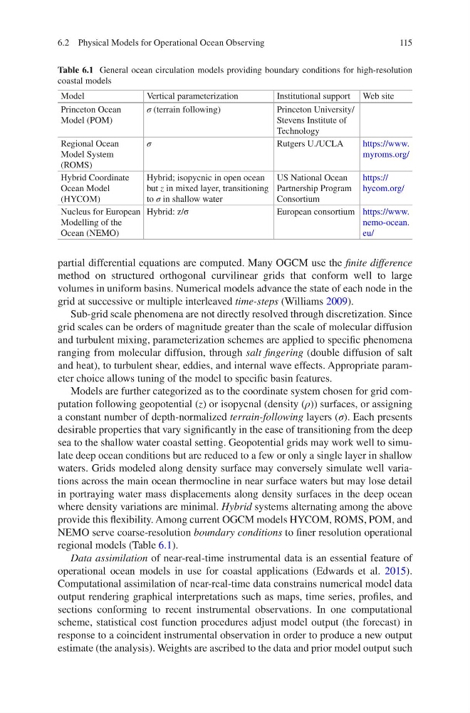
regional models (Table 6.1).
Data assimilation of near-real-time instrumental data is an essential feature of
operational ocean models in use for coastal applications (Edwards et al. 2015).
Computational assimilation of near-real-time data constrains numerical model data
output rendering graphical interpretations such as maps, time series, profiles, and
sections conforming to recent instrumental observations. In one computational
scheme, statistical cost function procedures adjust model output (the forecast) in
response to a coincident instrumental observation in order to produce a new output
estimate (the analysis). Weights are ascribed to the data and prior model output such
Table 6.1 General ocean circulation models providing boundary conditions for high-resolution
coastal models
Model
Vertical parameterization
Institutional support Web site
Princeton Ocean
Model (POM)
σ (terrain following)
Princeton University/
Stevens Institute of
Technology
Regional Ocean
Model System
(ROMS)
σ
Rutgers U./UCLA
https://www.
myroms.org/
Hybrid Coordinate
Ocean Model
(HYCOM)
Hybrid; isopycnic in open ocean
but z in mixed layer, transitioning
to σ in shallow water
US National Ocean
Partnership Program
Consortium
https://
hycom.org/
Nucleus for European
Modelling of the
Ocean (NEMO)
Hybrid: z/σ
European consortium https://www.
nemo-ocean.
eu/
6.2 Physical Models for Operational Ocean Observing
partial differential equations are computed. Many OGCM use the finite difference
method on structured orthogonal curvilinear grids that conform well to large
volumes in uniform basins. Numerical models advance the state of each node in the
grid at successive or multiple interleaved time-steps (Williams 2009).
Sub-grid scale phenomena are not directly resolved through discretization. Since
grid scales can be orders of magnitude greater than the scale of molecular diffusion
and turbulent mixing, parameterization schemes are applied to specific phenomena
ranging from molecular diffusion, through salt fingering (double diffusion of salt
and heat), to turbulent shear, eddies, and internal wave effects. Appropriate parameter choice allows tuning of the model to specific basin features.
Models are further categorized as to the coordinate system chosen for grid computation following geopotential (z) or isopycnal (density (ρ)) surfaces, or assigning
a constant number of depth-normalized terrain-following layers (σ). Each presents
desirable properties that vary significantly in the ease of transitioning from the deep
sea to the shallow water coastal setting. Geopotential grids may work well to simulate deep ocean conditions but are reduced to a few or only a single layer in shallow
waters. Grids modeled along density surface may conversely simulate well variations across the main ocean thermocline in near surface waters but may lose detail
in portraying water mass displacements along density surfaces in the deep ocean
where density variations are minimal. Hybrid systems alternating among the above
provide this flexibility. Among current OGCM models HYCOM, ROMS, POM, and
NEMO serve coarse-resolution boundary conditions to finer resolution operational
regional models (Table 6.1).
Data assimilation of near-real-time instrumental data is an essential feature of
operational ocean models in use for coastal applications (Edwards et al. 2015).
Computational assimilation of near-real-time data constrains numerical model data
output rendering graphical interpretations such as maps, time series, profiles, and
sections conforming to recent instrumental observations. In one computational
scheme, statistical cost function procedures adjust model output (the forecast) in
response to a coincident instrumental observation in order to produce a new output
estimate (the analysis). Weights are ascribed to the data and prior model output such
Table 6.1 General ocean circulation models providing boundary conditions for high-resolution
coastal models
Model
Vertical parameterization
Institutional support Web site
Princeton Ocean
Model (POM)
σ (terrain following)
Princeton University/
Stevens Institute of
Technology
Regional Ocean
Model System
(ROMS)
σ
Rutgers U./UCLA
https://www.
myroms.org/
Hybrid Coordinate
Ocean Model
(HYCOM)
Hybrid; isopycnic in open ocean
but z in mixed layer, transitioning
to σ in shallow water
US National Ocean
Partnership Program
Consortium
https://
hycom.org/
Nucleus for European
Modelling of the
Ocean (NEMO)
Hybrid: z/σ
European consortium https://www.
nemo-ocean.
eu/
6.2 Physical Models for Operational Ocean Observing