

349
Airborne Water Vapor Differential Absorption Lidar
layer to an altitude of 2.5–3.5 km by 0345 UTC (37.1°N shown in Figure 14.6). Three
distinct solitary waves were observed within the inversion surface. The crest-to-crest
spacing of the waves is 15 km. On the second overpass (0408–0427 UTC), NRL P-3
crossed over the bore at 0415 UTC. The same three waves appear in the data, with a
horizontal wavelength of 17 km. The waves are amplitude ordered, with the leading
one (the bore head) displaying a 0.7-km amplitude and the second and third ones
showing a 0.4-km amplitude (crest to trough). For the final overpass (0555–0616
UTC), the bore was passed at 0602 UTC. During this period, the ground-observing
systems at Homestead were also sampling this feature very intensively. The most
beautiful wave patterns on this day were captured by LEANDRE II with this pass
through what is apparently a very well-defined soliton composed of more than nine
waves, with a wave spacing of 11–12 km. Another interesting feature seen in this
display is that the amplitude ordering is no longer present; instead, the inversion
surface is lifted successfully higher by each passing wave, from 1.3 to 1.7 km MSL
with the first wave to eventually 2.1 km MSL by the fourth wave, after which the
depth of the layer remains essentially the same. This gives valuable information
about the length scale of the transition region and suggests an interesting hypothesis
that the demise of the soliton was brought about by the flattening of the leading
wave in the wave train. Also of considerable interest is the appearance of “ghost”
oscillations at a 3.2-km altitude in phase with those much lower. These features may
actually be cloud-induced lifting below that altitude. The lack of any vertical tilt
reveals that these are trapped waves occupying a deep layer from 1.3 to 3.3 km MSL.
Besides the wave patterns, other remarkable features observed by LEANDRE II
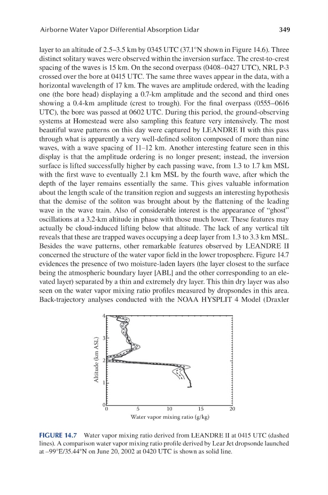
concerned the structure of the water vapor field in the lower troposphere. Figure 14.7
evidences the presence of two moisture-laden layers (the layer closest to the surface
being the atmospheric boundary layer [ABL] and the other corresponding to an elevated layer) separated by a thin and extremely dry layer. This thin dry layer was also
seen on the water vapor mixing ratio profiles measured by dropsondes in this area.
Back-trajectory analyses conducted with the NOAA HYSPLIT 4 Model (Draxler
4
3
2
1
0
0
5
10
15
20
Water vapor mixing ratio (g/kg)
Altitude (km ASL)
FIGURE 14.7 Water vapor mixing ratio derived from LEANDRE II at 0415 UTC (dashed
lines). A comparison water vapor mixing ratio profile derived by Lear Jet dropsonde launched
at –99°E/35.44°N on June 20, 2002 at 0420 UTC is shown as solid line.
Airborne Water Vapor Differential Absorption Lidar
layer to an altitude of 2.5–3.5 km by 0345 UTC (37.1°N shown in Figure 14.6). Three
distinct solitary waves were observed within the inversion surface. The crest-to-crest
spacing of the waves is 15 km. On the second overpass (0408–0427 UTC), NRL P-3
crossed over the bore at 0415 UTC. The same three waves appear in the data, with a
horizontal wavelength of 17 km. The waves are amplitude ordered, with the leading
one (the bore head) displaying a 0.7-km amplitude and the second and third ones
showing a 0.4-km amplitude (crest to trough). For the final overpass (0555–0616
UTC), the bore was passed at 0602 UTC. During this period, the ground-observing
systems at Homestead were also sampling this feature very intensively. The most
beautiful wave patterns on this day were captured by LEANDRE II with this pass
through what is apparently a very well-defined soliton composed of more than nine
waves, with a wave spacing of 11–12 km. Another interesting feature seen in this
display is that the amplitude ordering is no longer present; instead, the inversion
surface is lifted successfully higher by each passing wave, from 1.3 to 1.7 km MSL
with the first wave to eventually 2.1 km MSL by the fourth wave, after which the
depth of the layer remains essentially the same. This gives valuable information
about the length scale of the transition region and suggests an interesting hypothesis
that the demise of the soliton was brought about by the flattening of the leading
wave in the wave train. Also of considerable interest is the appearance of “ghost”
oscillations at a 3.2-km altitude in phase with those much lower. These features may
actually be cloud-induced lifting below that altitude. The lack of any vertical tilt
reveals that these are trapped waves occupying a deep layer from 1.3 to 3.3 km MSL.
Besides the wave patterns, other remarkable features observed by LEANDRE II
concerned the structure of the water vapor field in the lower troposphere. Figure 14.7
evidences the presence of two moisture-laden layers (the layer closest to the surface
being the atmospheric boundary layer [ABL] and the other corresponding to an elevated layer) separated by a thin and extremely dry layer. This thin dry layer was also
seen on the water vapor mixing ratio profiles measured by dropsondes in this area.
Back-trajectory analyses conducted with the NOAA HYSPLIT 4 Model (Draxler
4
3
2
1
0
0
5
10
15
20
Water vapor mixing ratio (g/kg)
Altitude (km ASL)
FIGURE 14.7 Water vapor mixing ratio derived from LEANDRE II at 0415 UTC (dashed
lines). A comparison water vapor mixing ratio profile derived by Lear Jet dropsonde launched
at –99°E/35.44°N on June 20, 2002 at 0420 UTC is shown as solid line.