

317
Radar Polarimetry for Rain Estimation
where Z DR
up
Z DR
low
( ) denotes the upper (lower) boundary. Equation 13.19 implies that,
if an observed Z DR deviates from the normal range of rain data, Z DR would be less
reliable in representing rain.
The procedure for Bayesian retrieval is briefly described below. Given the radar
measurements Z H and Z DR , the conditional probability can be calculated by Equations
13.18 and 13.19. Knowing the a priori PDF of DSD parameters, mean values and
standard deviations of DSD parameters are retrieved by applying Equations 13.16
and 13.17. Next, the gamma DSD is constructed using retrieved mean values. Finally,
rain variables of interest can be calculated from the retrieved gamma DSD.
13.3.2.2.3 Variational Approach
A storm normally has a spatial dependence attributed to the physical process of its
evolution. As a result, radar measurements of a storm would have a spatial correlation, which can be used to minimize the measurement error. A variational scheme
not only considers qualities and reliabilities of different radar measurements but also
utilizes the spatial information to optimize the retrieval (Ide et al. 1997). Multiple
observations can be easily balanced with error-based weighting and optimally used
in the scheme. Attenuation correction can be embedded into the forward observation
operator and optimized as well. Some studies (e.g., Hogan 2007; Xue et al. 2009)
applied radar measurements in a variational scheme for the retrieval of integral
parameters such as rainfall rate. Since the DSD is of greater interest, a variational
scheme can be introduced below for the retrieval of DSD parameters to show the
basic concept of the variational approach.
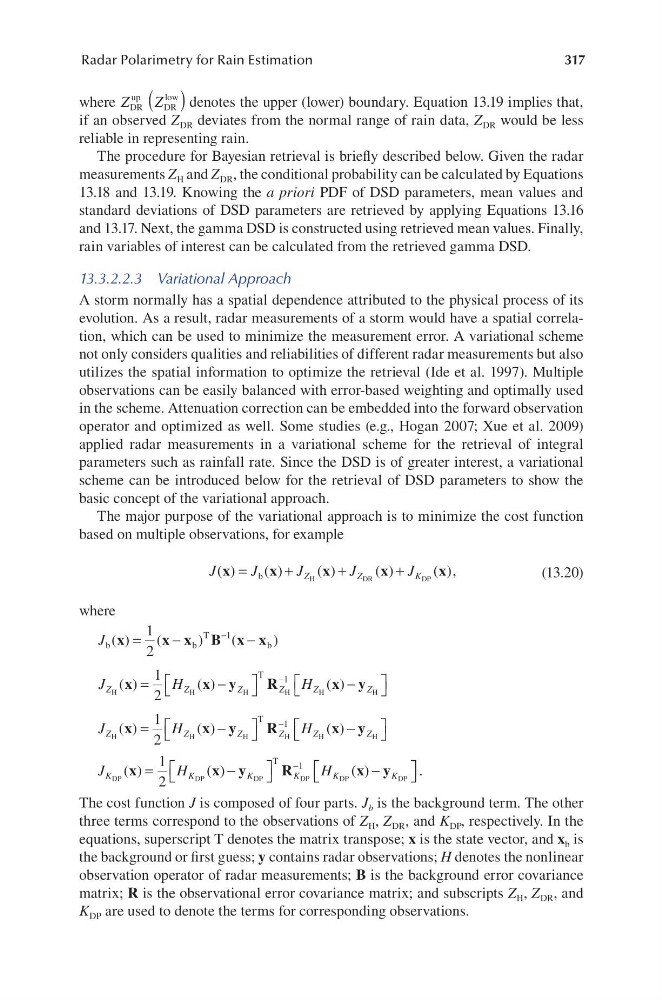
The major purpose of the variational approach is to minimize the cost function
based on multiple observations, for example
J
J
J
J
J
Z
Z
K
( )
( )
( )
( )
( )
x
x
x
x
x
=
+
+
+
b
H
DR
DP
,
(13.20)
where
J b
b
T
b
( )
(
)
(
)
x
x x B x x
=
−
−
−
1
2
1
J
H
H
Z
Z
Z
Z
Z
Z
H
H
H
H
H
H
T
( )
( )
( )
x
x y
R
x y
=
−
−
−
1
2
1
J
H
H
Z
Z
Z
Z
Z
Z
H
H
H
H
H
H
T
( )
( )
( )
x
x y
R
x y
=
−
−
−
1
2
1
J
H
H
K
K
K
K
K
K
DP
DP
DP
DP
DP
DP
T
( )
( )
( )
x
x y
R
x y
=
−
−
−
1
2
1
.
The cost function J is composed of four parts. J b is the background term. The other
three terms correspond to the observations of Z H , Z DR , and K DP , respectively. In the
equations, superscript T denotes the matrix transpose; x is the state vector, and x b is
the background or first guess; y contains radar observations; H denotes the nonlinear
observation operator of radar measurements; B is the background error covariance
matrix; R is the observational error covariance matrix; and subscripts Z H , Z DR , and
K DP are used to denote the terms for corresponding observations.
Radar Polarimetry for Rain Estimation
where Z DR
up
Z DR
low
( ) denotes the upper (lower) boundary. Equation 13.19 implies that,
if an observed Z DR deviates from the normal range of rain data, Z DR would be less
reliable in representing rain.
The procedure for Bayesian retrieval is briefly described below. Given the radar
measurements Z H and Z DR , the conditional probability can be calculated by Equations
13.18 and 13.19. Knowing the a priori PDF of DSD parameters, mean values and
standard deviations of DSD parameters are retrieved by applying Equations 13.16
and 13.17. Next, the gamma DSD is constructed using retrieved mean values. Finally,
rain variables of interest can be calculated from the retrieved gamma DSD.
13.3.2.2.3 Variational Approach
A storm normally has a spatial dependence attributed to the physical process of its
evolution. As a result, radar measurements of a storm would have a spatial correlation, which can be used to minimize the measurement error. A variational scheme
not only considers qualities and reliabilities of different radar measurements but also
utilizes the spatial information to optimize the retrieval (Ide et al. 1997). Multiple
observations can be easily balanced with error-based weighting and optimally used
in the scheme. Attenuation correction can be embedded into the forward observation
operator and optimized as well. Some studies (e.g., Hogan 2007; Xue et al. 2009)
applied radar measurements in a variational scheme for the retrieval of integral
parameters such as rainfall rate. Since the DSD is of greater interest, a variational
scheme can be introduced below for the retrieval of DSD parameters to show the
basic concept of the variational approach.
The major purpose of the variational approach is to minimize the cost function
based on multiple observations, for example
J
J
J
J
J
Z
Z
K
( )
( )
( )
( )
( )
x
x
x
x
x
=
+
+
+
b
H
DR
DP
,
(13.20)
where
J b
b
T
b
( )
(
)
(
)
x
x x B x x
=
−
−
−
1
2
1
J
H
H
Z
Z
Z
Z
Z
Z
H
H
H
H
H
H
T
( )
( )
( )
x
x y
R
x y
=
−
−
−
1
2
1
J
H
H
Z
Z
Z
Z
Z
Z
H
H
H
H
H
H
T
( )
( )
( )
x
x y
R
x y
=
−
−
−
1
2
1
J
H
H
K
K
K
K
K
K
DP
DP
DP
DP
DP
DP
T
( )
( )
( )
x
x y
R
x y
=
−
−
−
1
2
1
.
The cost function J is composed of four parts. J b is the background term. The other
three terms correspond to the observations of Z H , Z DR , and K DP , respectively. In the
equations, superscript T denotes the matrix transpose; x is the state vector, and x b is
the background or first guess; y contains radar observations; H denotes the nonlinear
observation operator of radar measurements; B is the background error covariance
matrix; R is the observational error covariance matrix; and subscripts Z H , Z DR , and
K DP are used to denote the terms for corresponding observations.