

312
Multiscale Hydrologic Remote Sensing: Perspectives and Applications
also frequency dependent. Compared with the empirical approach, DSD retrieval is
more flexible for the application of measurements on different radar platforms.
13.3.2 dSd-BaSed RetRievalS
13.3.2.1 DSD Models
DSD provides fundamental information on rain microphysics. If the DSD is known,
all rain variables can be derived through DSD integration (as shown in Equations
13.5 through 13.8). There are some popular relations to model a DSD in the meteo3.5 through 13.8). There are some popular relations to model a DSD in the meteo.5 through 13.8). There are some popular relations to model a DSD in the meteo3.8). There are some popular relations to model a DSD in the meteo.8). There are some popular relations to model a DSD in the meteorological community. Marshall and Palmer (1948) proposed the well-known M–P
model, N(D) = 8000exp(–ΛD), which has been used widely in the last 50 years. It is
a single-parameter model with a slope parameter Λ. It was helpful in bulk-scheme
rain parameterization and radar–rain estimation when single-polarization weather
radars prevailed. Later, the exponential model, N(D) = N 0 exp(–ΛD), was applied.
It is a two-parameter model with an additional concentration parameter, N 0 . It is
more flexible than the M–P model, since the latter is equivalent to the exponential
model with a fixed N 0 . It can be applied for dual-frequency/dual-polarization weather
radars. Ulbrich (1983) introduced the gamma model as
N(D) = N 0 D μ exp(–ΛD).
(13.12)
Compared with the exponential model, Equation 13.12 includes a third parameter,
shape μ. It has been widely accepted that the gamma model can represent well the
variability of natural DSDs. Some recent studies applied the normalized gamma
DSD (Bringi et al. 2002).
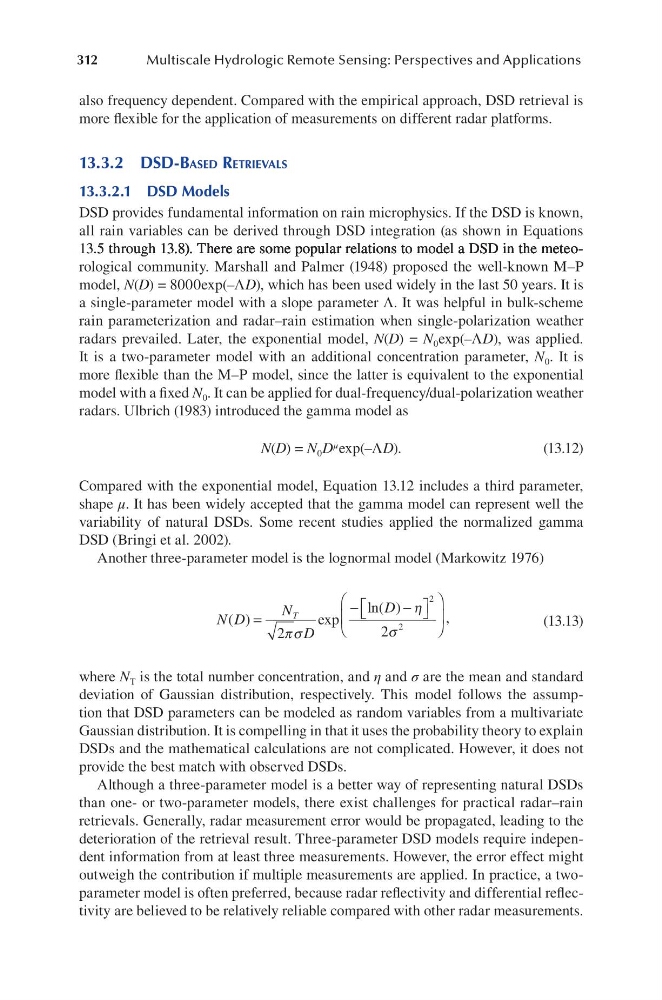
Another three-parameter model is the lognormal model (Markowitz 1976)
N D
N
D
D
T
( )
exp
ln( )
=
−
−
2
2
2
2
π σ
η
σ
,
(13.13)
where N T is the total number concentration, and η and σ are the mean and standard
deviation of Gaussian distribution, respectively. This model follows the assumption that DSD parameters can be modeled as random variables from a multivariate
Gaussian distribution. It is compelling in that it uses the probability theory to explain
DSDs and the mathematical calculations are not complicated. However, it does not
provide the best match with observed DSDs.
Although a three-parameter model is a better way of representing natural DSDs
than one- or two-parameter models, there exist challenges for practical radar–rain
retrievals. Generally, radar measurement error would be propagated, leading to the
deterioration of the retrieval result. Three-parameter DSD models require independent information from at least three measurements. However, the error effect might
outweigh the contribution if multiple measurements are applied. In practice, a twoparameter model is often preferred, because radar reflectivity and differential reflectivity are believed to be relatively reliable compared with other radar measurements.
Multiscale Hydrologic Remote Sensing: Perspectives and Applications
also frequency dependent. Compared with the empirical approach, DSD retrieval is
more flexible for the application of measurements on different radar platforms.
13.3.2 dSd-BaSed RetRievalS
13.3.2.1 DSD Models
DSD provides fundamental information on rain microphysics. If the DSD is known,
all rain variables can be derived through DSD integration (as shown in Equations
13.5 through 13.8). There are some popular relations to model a DSD in the meteo3.5 through 13.8). There are some popular relations to model a DSD in the meteo.5 through 13.8). There are some popular relations to model a DSD in the meteo3.8). There are some popular relations to model a DSD in the meteo.8). There are some popular relations to model a DSD in the meteorological community. Marshall and Palmer (1948) proposed the well-known M–P
model, N(D) = 8000exp(–ΛD), which has been used widely in the last 50 years. It is
a single-parameter model with a slope parameter Λ. It was helpful in bulk-scheme
rain parameterization and radar–rain estimation when single-polarization weather
radars prevailed. Later, the exponential model, N(D) = N 0 exp(–ΛD), was applied.
It is a two-parameter model with an additional concentration parameter, N 0 . It is
more flexible than the M–P model, since the latter is equivalent to the exponential
model with a fixed N 0 . It can be applied for dual-frequency/dual-polarization weather
radars. Ulbrich (1983) introduced the gamma model as
N(D) = N 0 D μ exp(–ΛD).
(13.12)
Compared with the exponential model, Equation 13.12 includes a third parameter,
shape μ. It has been widely accepted that the gamma model can represent well the
variability of natural DSDs. Some recent studies applied the normalized gamma
DSD (Bringi et al. 2002).
Another three-parameter model is the lognormal model (Markowitz 1976)
N D
N
D
D
T
( )
exp
ln( )
=
−
−
2
2
2
2
π σ
η
σ
,
(13.13)
where N T is the total number concentration, and η and σ are the mean and standard
deviation of Gaussian distribution, respectively. This model follows the assumption that DSD parameters can be modeled as random variables from a multivariate
Gaussian distribution. It is compelling in that it uses the probability theory to explain
DSDs and the mathematical calculations are not complicated. However, it does not
provide the best match with observed DSDs.
Although a three-parameter model is a better way of representing natural DSDs
than one- or two-parameter models, there exist challenges for practical radar–rain
retrievals. Generally, radar measurement error would be propagated, leading to the
deterioration of the retrieval result. Three-parameter DSD models require independent information from at least three measurements. However, the error effect might
outweigh the contribution if multiple measurements are applied. In practice, a twoparameter model is often preferred, because radar reflectivity and differential reflectivity are believed to be relatively reliable compared with other radar measurements.