

310
Multiscale Hydrologic Remote Sensing: Perspectives and Applications
estimators, which are evaluated by Ryzhkov et al. (2005a). These empirical relations
are specific for S-band applications.
Bringi and Chandrasekar (2001) gave a detailed analysis of estimation error for
empirical polarimetric estimators. There are different error structures for those estimators. Polarimetric estimators have their own advantages and disadvantages. For
example, when rain is intense and/or mixed with hail, K DP generally has a better
representation of rain physics. In that case, R(K DP ) normally has a small error of rain
estimation. However, when rain is light, the measurement error of K DP is relatively
large, and it is not appropriate to apply R(K DP ). Ryzhkov et al. (2005a) show a “synthetic” approach, applying R(Z h ,Z dr ), R(K DP ), and R(K DP ,Z dr ), with a minor difference
from power-law forms, in three different ranges of rainfall rate. For R < 6 mm –1 ,
R(Z h ,Z dr ) is applied; for R > 50 mm –1 , R(K DP ) is applied; and R(K DP ,Z dr ) is applied for
other cases.
Figure 13.2 shows the rain retrievals using different estimators for radar measure3.2 shows the rain retrievals using different estimators for radar measure.2 shows the rain retrievals using different estimators for radar measurements shown in Figure 13.1. Figure 13.2a to c gives the results of three empirical
estimators, which are developed by the NSSL. R = 0.017Z h
0.714 is a default estimator
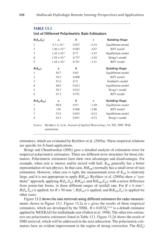
applied by NEXRAD for midlatitude rain (Fulton et al. 1998). The other two estimators are polarimetric estimators listed in Table 13.1. Figure 13.2d shows the result of
DSD retrieval, which will be addressed in the next subsection. The polarimetric estimators have an evident improvement in the region of strong convection. The R(Z h )
TABLE 13.1
List of Different Polarimetric Rain Estimators
r(Z h ,Z dr )
a
b
c
Raindrop Shape
1
6.7 × 10 –3
0.927
–3.43
Equilibrium model
2
7.46 × 10 –3
0.945
–4.67
BZV model
3
1.42 × 10 –2
0.77
–1.67
Equilibrium model
4
1.59 × 10 –2
0.737
–1.03
Bringi’s model
5
1.44 × 10 –2
0.761
–1.51
BZV model
r(K DP )
a
b
Raindrop Shape
1
50.7
0.85
Equilibrium model
2
54.3
0.806
BZV model
3
51.6
0.71
Goddard’s model
4
44.0
0.822
Equilibrium model
5
50.3
0.812
Bringi’s model
6
47.3
0.791
BZV model
r(Z dr ,K DP )
a
b
c
Raindrop Shape
1
90.8
0.93
–1.69
Equilibrium model
2
136
0.968
–2.86
BZV model
3
52.9
0.852
–0.53
Equilibrium model
4
63.3
0.851
–0.72
Bringi’s model
Source: Ryzhkov, A. et al., Journal of Applied Meteorology, 44, 502, 2005. With
permission.
Multiscale Hydrologic Remote Sensing: Perspectives and Applications
estimators, which are evaluated by Ryzhkov et al. (2005a). These empirical relations
are specific for S-band applications.
Bringi and Chandrasekar (2001) gave a detailed analysis of estimation error for
empirical polarimetric estimators. There are different error structures for those estimators. Polarimetric estimators have their own advantages and disadvantages. For
example, when rain is intense and/or mixed with hail, K DP generally has a better
representation of rain physics. In that case, R(K DP ) normally has a small error of rain
estimation. However, when rain is light, the measurement error of K DP is relatively
large, and it is not appropriate to apply R(K DP ). Ryzhkov et al. (2005a) show a “synthetic” approach, applying R(Z h ,Z dr ), R(K DP ), and R(K DP ,Z dr ), with a minor difference
from power-law forms, in three different ranges of rainfall rate. For R < 6 mm –1 ,
R(Z h ,Z dr ) is applied; for R > 50 mm –1 , R(K DP ) is applied; and R(K DP ,Z dr ) is applied for
other cases.
Figure 13.2 shows the rain retrievals using different estimators for radar measure3.2 shows the rain retrievals using different estimators for radar measure.2 shows the rain retrievals using different estimators for radar measurements shown in Figure 13.1. Figure 13.2a to c gives the results of three empirical
estimators, which are developed by the NSSL. R = 0.017Z h
0.714 is a default estimator
applied by NEXRAD for midlatitude rain (Fulton et al. 1998). The other two estimators are polarimetric estimators listed in Table 13.1. Figure 13.2d shows the result of
DSD retrieval, which will be addressed in the next subsection. The polarimetric estimators have an evident improvement in the region of strong convection. The R(Z h )
TABLE 13.1
List of Different Polarimetric Rain Estimators
r(Z h ,Z dr )
a
b
c
Raindrop Shape
1
6.7 × 10 –3
0.927
–3.43
Equilibrium model
2
7.46 × 10 –3
0.945
–4.67
BZV model
3
1.42 × 10 –2
0.77
–1.67
Equilibrium model
4
1.59 × 10 –2
0.737
–1.03
Bringi’s model
5
1.44 × 10 –2
0.761
–1.51
BZV model
r(K DP )
a
b
Raindrop Shape
1
50.7
0.85
Equilibrium model
2
54.3
0.806
BZV model
3
51.6
0.71
Goddard’s model
4
44.0
0.822
Equilibrium model
5
50.3
0.812
Bringi’s model
6
47.3
0.791
BZV model
r(Z dr ,K DP )
a
b
c
Raindrop Shape
1
90.8
0.93
–1.69
Equilibrium model
2
136
0.968
–2.86
BZV model
3
52.9
0.852
–0.53
Equilibrium model
4
63.3
0.851
–0.72
Bringi’s model
Source: Ryzhkov, A. et al., Journal of Applied Meteorology, 44, 502, 2005. With
permission.