

133
Spatiotemporal Interactions among Ecohydrological Factors
observed low ET pattern in the wet season (see Figure 6.5). These concomitant soil
moisture patterns and ET fluctuations vary among urban patches from downtown to
rural areas and closely follow the urban gradient. Land with less vegetation cover has a
poorer capacity to store rain water. Compared to the LULC maps (Figure 6.1a), higher
soil moistures corresponded to the wetlands in the Hillsborough River and Alafia River
Basin area, as well as cultivated crops in the Manatee River and Little Manatee River
Basin area. Compared with the EVI values, the ET values from May 2005 to April 2006
in the study area (Figure 6.5) look more varied and sensitive, and they soared in July.
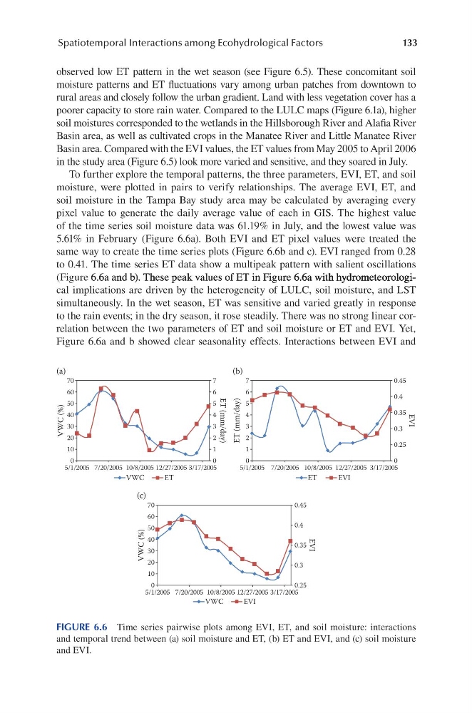
To further explore the temporal patterns, the three parameters, EVI, ET, and soil
moisture, were plotted in pairs to verify relationships. The average EVI, ET, and
soil moisture in the Tampa Bay study area may be calculated by averaging every
pixel value to generate the daily average value of each in GIS. The highest value
of the time series soil moisture data was 61.19% in July, and the lowest value was
5.61% in February (Figure 6.6a). Both EVI and ET pixel values were treated the
same way to create the time series plots (Figure 6.6b and c). EVI ranged from 0.28
to 0.41. The time series ET data show a multipeak pattern with salient oscillations
(Figure 6.6a and b). These peak values of ET in Figure 6.6a with hydrometeorologi6.6a and b). These peak values of ET in Figure 6.6a with hydrometeorologi.6a and b). These peak values of ET in Figure 6.6a with hydrometeorologi6.6a with hydrometeorologi.6a with hydrometeorological implications are driven by the heterogeneity of LULC, soil moisture, and LST
simultaneously. In the wet season, ET was sensitive and varied greatly in response
to the rain events; in the dry season, it rose steadily. There was no strong linear correlation between the two parameters of ET and soil moisture or ET and EVI. Yet,
Figure 6.6a and b showed clear seasonality effects. Interactions between EVI and
70
60
50
40
30
20
10
0
5/1/2005
VWC (%)
ET (mm/day)
7/20/2005 10/8/2005 12/27/2005 3/17/2005
7
6
5
4
3
2
1
0
70
60
50
40
30
20
10
0
5/1/2005
VWC (%)
EVI
7/20/2005 10/8/2005 12/27/2005 3/17/2005
0.45
0.4
0.35
0.3
0.25
7
6
5
4
3
2
1
0
5/1/2005
ET (mm/day)
EVI
7/20/2005 10/8/2005 12/27/2005 3/17/2005
0.45
0.4
0.35
0.3
0.25
0
VWC
ET
VWC
EVI
ET
EVI
(a)
(b)
(c)
FIGURE 6.6 Time series pairwise plots among EVI, ET, and soil moisture: interactions
and temporal trend between (a) soil moisture and ET, (b) ET and EVI, and (c) soil moisture
and EVI.
Spatiotemporal Interactions among Ecohydrological Factors
observed low ET pattern in the wet season (see Figure 6.5). These concomitant soil
moisture patterns and ET fluctuations vary among urban patches from downtown to
rural areas and closely follow the urban gradient. Land with less vegetation cover has a
poorer capacity to store rain water. Compared to the LULC maps (Figure 6.1a), higher
soil moistures corresponded to the wetlands in the Hillsborough River and Alafia River
Basin area, as well as cultivated crops in the Manatee River and Little Manatee River
Basin area. Compared with the EVI values, the ET values from May 2005 to April 2006
in the study area (Figure 6.5) look more varied and sensitive, and they soared in July.
To further explore the temporal patterns, the three parameters, EVI, ET, and soil
moisture, were plotted in pairs to verify relationships. The average EVI, ET, and
soil moisture in the Tampa Bay study area may be calculated by averaging every
pixel value to generate the daily average value of each in GIS. The highest value
of the time series soil moisture data was 61.19% in July, and the lowest value was
5.61% in February (Figure 6.6a). Both EVI and ET pixel values were treated the
same way to create the time series plots (Figure 6.6b and c). EVI ranged from 0.28
to 0.41. The time series ET data show a multipeak pattern with salient oscillations
(Figure 6.6a and b). These peak values of ET in Figure 6.6a with hydrometeorologi6.6a and b). These peak values of ET in Figure 6.6a with hydrometeorologi.6a and b). These peak values of ET in Figure 6.6a with hydrometeorologi6.6a with hydrometeorologi.6a with hydrometeorological implications are driven by the heterogeneity of LULC, soil moisture, and LST
simultaneously. In the wet season, ET was sensitive and varied greatly in response
to the rain events; in the dry season, it rose steadily. There was no strong linear correlation between the two parameters of ET and soil moisture or ET and EVI. Yet,
Figure 6.6a and b showed clear seasonality effects. Interactions between EVI and
70
60
50
40
30
20
10
0
5/1/2005
VWC (%)
ET (mm/day)
7/20/2005 10/8/2005 12/27/2005 3/17/2005
7
6
5
4
3
2
1
0
70
60
50
40
30
20
10
0
5/1/2005
VWC (%)
EVI
7/20/2005 10/8/2005 12/27/2005 3/17/2005
0.45
0.4
0.35
0.3
0.25
7
6
5
4
3
2
1
0
5/1/2005
ET (mm/day)
EVI
7/20/2005 10/8/2005 12/27/2005 3/17/2005
0.45
0.4
0.35
0.3
0.25
0
VWC
ET
VWC
EVI
ET
EVI
(a)
(b)
(c)
FIGURE 6.6 Time series pairwise plots among EVI, ET, and soil moisture: interactions
and temporal trend between (a) soil moisture and ET, (b) ET and EVI, and (c) soil moisture
and EVI.