

116
Multiscale Hydrologic Remote Sensing: Perspectives and Applications
signal, and a reduction in atmosphere influences (Huete et al. 1999). The values of
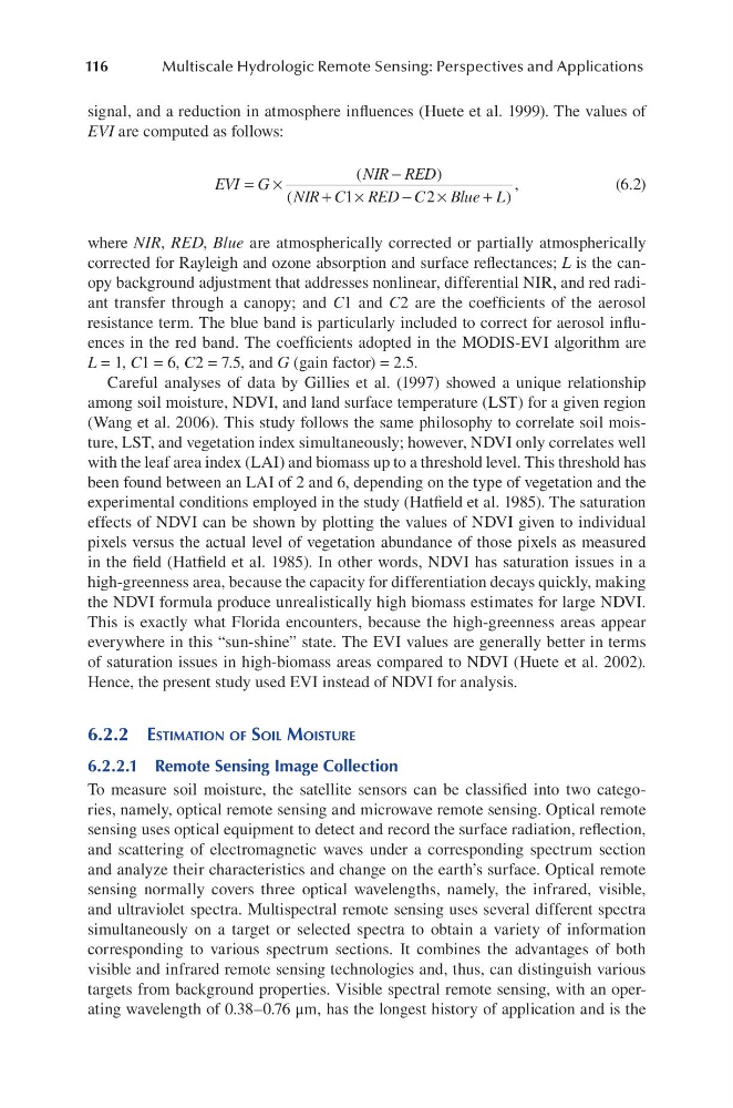
EVI are computed as follows:
EVI G
NIR RED
NIR C RED C
Blue L
= ×
−
+ ×
−
×
+
(
)
(
)
,
1
2
(6.2)
where NIR, RED, Blue are atmospherically corrected or partially atmospherically
corrected for Rayleigh and ozone absorption and surface reflectances; L is the canopy background adjustment that addresses nonlinear, differential NIR, and red radiant transfer through a canopy; and C1 and C2 are the coefficients of the aerosol
resistance term. The blue band is particularly included to correct for aerosol influences in the red band. The coefficients adopted in the MODIS-EVI algorithm are
L = 1, C1 = 6, C2 = 7.5, and G (gain factor) = 2.5.
Careful analyses of data by Gillies et al. (1997) showed a unique relationship
among soil moisture, NDVI, and land surface temperature (LST) for a given region
(Wang et al. 2006). This study follows the same philosophy to correlate soil moisture, LST, and vegetation index simultaneously; however, NDVI only correlates well
with the leaf area index (LAI) and biomass up to a threshold level. This threshold has
been found between an LAI of 2 and 6, depending on the type of vegetation and the
experimental conditions employed in the study (Hatfield et al. 1985). The saturation
effects of NDVI can be shown by plotting the values of NDVI given to individual
pixels versus the actual level of vegetation abundance of those pixels as measured
in the field (Hatfield et al. 1985). In other words, NDVI has saturation issues in a
high-greenness area, because the capacity for differentiation decays quickly, making
the NDVI formula produce unrealistically high biomass estimates for large NDVI.
This is exactly what Florida encounters, because the high-greenness areas appear
everywhere in this “sun-shine” state. The EVI values are generally better in terms
of saturation issues in high-biomass areas compared to NDVI (Huete et al. 2002).
Hence, the present study used EVI instead of NDVI for analysis.
6.2.2 eStiMation of Soil MoiStuRe
6.2.2.1 Remote Sensing Image Collection
To measure soil moisture, the satellite sensors can be classified into two categories, namely, optical remote sensing and microwave remote sensing. Optical remote
sensing uses optical equipment to detect and record the surface radiation, reflection,
and scattering of electromagnetic waves under a corresponding spectrum section
and analyze their characteristics and change on the earth’s surface. Optical remote
sensing normally covers three optical wavelengths, namely, the infrared, visible,
and ultraviolet spectra. Multispectral remote sensing uses several different spectra
simultaneously on a target or selected spectra to obtain a variety of information
corresponding to various spectrum sections. It combines the advantages of both
visible and infrared remote sensing technologies and, thus, can distinguish various
targets from background properties. Visible spectral remote sensing, with an operating wavelength of 0.38–0.76 μm, has the longest history of application and is the
Multiscale Hydrologic Remote Sensing: Perspectives and Applications
signal, and a reduction in atmosphere influences (Huete et al. 1999). The values of
EVI are computed as follows:
EVI G
NIR RED
NIR C RED C
Blue L
= ×
−
+ ×
−
×
+
(
)
(
)
,
1
2
(6.2)
where NIR, RED, Blue are atmospherically corrected or partially atmospherically
corrected for Rayleigh and ozone absorption and surface reflectances; L is the canopy background adjustment that addresses nonlinear, differential NIR, and red radiant transfer through a canopy; and C1 and C2 are the coefficients of the aerosol
resistance term. The blue band is particularly included to correct for aerosol influences in the red band. The coefficients adopted in the MODIS-EVI algorithm are
L = 1, C1 = 6, C2 = 7.5, and G (gain factor) = 2.5.
Careful analyses of data by Gillies et al. (1997) showed a unique relationship
among soil moisture, NDVI, and land surface temperature (LST) for a given region
(Wang et al. 2006). This study follows the same philosophy to correlate soil moisture, LST, and vegetation index simultaneously; however, NDVI only correlates well
with the leaf area index (LAI) and biomass up to a threshold level. This threshold has
been found between an LAI of 2 and 6, depending on the type of vegetation and the
experimental conditions employed in the study (Hatfield et al. 1985). The saturation
effects of NDVI can be shown by plotting the values of NDVI given to individual
pixels versus the actual level of vegetation abundance of those pixels as measured
in the field (Hatfield et al. 1985). In other words, NDVI has saturation issues in a
high-greenness area, because the capacity for differentiation decays quickly, making
the NDVI formula produce unrealistically high biomass estimates for large NDVI.
This is exactly what Florida encounters, because the high-greenness areas appear
everywhere in this “sun-shine” state. The EVI values are generally better in terms
of saturation issues in high-biomass areas compared to NDVI (Huete et al. 2002).
Hence, the present study used EVI instead of NDVI for analysis.
6.2.2 eStiMation of Soil MoiStuRe
6.2.2.1 Remote Sensing Image Collection
To measure soil moisture, the satellite sensors can be classified into two categories, namely, optical remote sensing and microwave remote sensing. Optical remote
sensing uses optical equipment to detect and record the surface radiation, reflection,
and scattering of electromagnetic waves under a corresponding spectrum section
and analyze their characteristics and change on the earth’s surface. Optical remote
sensing normally covers three optical wavelengths, namely, the infrared, visible,
and ultraviolet spectra. Multispectral remote sensing uses several different spectra
simultaneously on a target or selected spectra to obtain a variety of information
corresponding to various spectrum sections. It combines the advantages of both
visible and infrared remote sensing technologies and, thus, can distinguish various
targets from background properties. Visible spectral remote sensing, with an operating wavelength of 0.38–0.76 μm, has the longest history of application and is the