

102
Multiscale Hydrologic Remote Sensing: Perspectives and Applications
thus decreasing the air temperature while increasing the water vapor concentration
resulting from continued evaporation in the absence of significant available energy
(R n – G).
Figure 5.7 shows T and ρ v for the same day but under unstable conditions at 1300
h. Here, we observe temperature and water vapor concentrations to be strongly correlated. Increases in temperature match increases in water vapor concentrations. Under
unstable conditions, the available energy is now the dominant source of energy for
evaporation to proceed to where approximately 90% of the available energy is consumed by evaporation, while the remaining available energy is partitioned into a
positive H (i.e., away from the surface). Both Figures 5.6 and 5.7 demonstrate how
well coupled the surface becomes to the overlying boundary layer under different
conditions of stability and advection of saturation deficit. Up and down drafts are
very well correlated, indicating a well-mixed layer as the mean wind flow traverses
across the irrigated cotton field. Figure 5.6 shows how increasing temperatures are
closely matched with increasing water vapor concentration when warmer drier air is
added to the volume of air space over the irrigated surface and the additional saturation deficit acts to increase the vapor pressure gradient, thus increasing evaporation
from the wet surface.
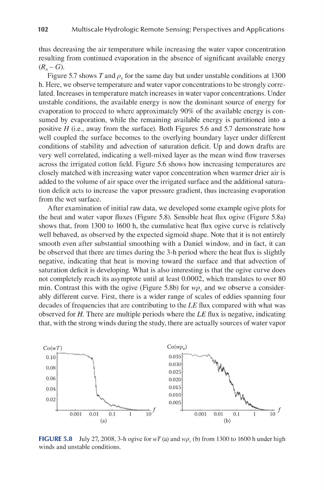
After examination of initial raw data, we developed some example ogive plots for
the heat and water vapor fluxes (Figure 5.8). Sensible heat flux ogive (Figure 5.8a)
shows that, from 1300 to 1600 h, the cumulative heat flux ogive curve is relatively
well behaved, as observed by the expected sigmoid shape. Note that it is not entirely
smooth even after substantial smoothing with a Daniel window, and in fact, it can
be observed that there are times during the 3-h period where the heat flux is slightly
negative, indicating that heat is moving toward the surface and that advection of
saturation deficit is developing. What is also interesting is that the ogive curve does
not completely reach its asymptote until at least 0.0002, which translates to over 80
min. Contrast this with the ogive (Figure 5.8b) for wρ v and we observe a considerably different curve. First, there is a wider range of scales of eddies spanning four
decades of frequencies that are contributing to the LE flux compared with what was
observed for H. There are multiple periods where the LE flux is negative, indicating
that, with the strong winds during the study, there are actually sources of water vapor
0.10
Co(wT )
Co(wρ v )
f
f
0.06
0.08
0.035
0.030
0.025
0.020
0.015
0.010
0.005
0.04
0.02
0.001 0.01
0.1
1
10
0.001 0.01
0.1
1
10
(a)
(b)
FIGURE 5.8 July 27, 2008, 3-h ogive for wT (a) and wρ v (b) from 1300 to 1600 h under high
winds and unstable conditions.
Multiscale Hydrologic Remote Sensing: Perspectives and Applications
thus decreasing the air temperature while increasing the water vapor concentration
resulting from continued evaporation in the absence of significant available energy
(R n – G).
Figure 5.7 shows T and ρ v for the same day but under unstable conditions at 1300
h. Here, we observe temperature and water vapor concentrations to be strongly correlated. Increases in temperature match increases in water vapor concentrations. Under
unstable conditions, the available energy is now the dominant source of energy for
evaporation to proceed to where approximately 90% of the available energy is consumed by evaporation, while the remaining available energy is partitioned into a
positive H (i.e., away from the surface). Both Figures 5.6 and 5.7 demonstrate how
well coupled the surface becomes to the overlying boundary layer under different
conditions of stability and advection of saturation deficit. Up and down drafts are
very well correlated, indicating a well-mixed layer as the mean wind flow traverses
across the irrigated cotton field. Figure 5.6 shows how increasing temperatures are
closely matched with increasing water vapor concentration when warmer drier air is
added to the volume of air space over the irrigated surface and the additional saturation deficit acts to increase the vapor pressure gradient, thus increasing evaporation
from the wet surface.
After examination of initial raw data, we developed some example ogive plots for
the heat and water vapor fluxes (Figure 5.8). Sensible heat flux ogive (Figure 5.8a)
shows that, from 1300 to 1600 h, the cumulative heat flux ogive curve is relatively
well behaved, as observed by the expected sigmoid shape. Note that it is not entirely
smooth even after substantial smoothing with a Daniel window, and in fact, it can
be observed that there are times during the 3-h period where the heat flux is slightly
negative, indicating that heat is moving toward the surface and that advection of
saturation deficit is developing. What is also interesting is that the ogive curve does
not completely reach its asymptote until at least 0.0002, which translates to over 80
min. Contrast this with the ogive (Figure 5.8b) for wρ v and we observe a considerably different curve. First, there is a wider range of scales of eddies spanning four
decades of frequencies that are contributing to the LE flux compared with what was
observed for H. There are multiple periods where the LE flux is negative, indicating
that, with the strong winds during the study, there are actually sources of water vapor
0.10
Co(wT )
Co(wρ v )
f
f
0.06
0.08
0.035
0.030
0.025
0.020
0.015
0.010
0.005
0.04
0.02
0.001 0.01
0.1
1
10
0.001 0.01
0.1
1
10
(a)
(b)
FIGURE 5.8 July 27, 2008, 3-h ogive for wT (a) and wρ v (b) from 1300 to 1600 h under high
winds and unstable conditions.