

4 Isotope Geochemistry in the Environment
69
the evaporated phase, while the heavier isotope 1sO remains in the remaining river
water leading to higher 5lso during the Summer (see also Sect. 2.4). The
significant differences between the isotopic compositions of groundwater and
river water allow us to quantify the sequence of exchange between the two
systems. Let us look again at the schematic diagram of Fig. 4.15. The trace
element concentrations in drinking water from a freshwater spring are dependent
on the trace concentrations in both groundwater and river water, the relative
amount that both water systems make up of the whole and the flow rate into the
drinking water reservoir. The flow rate at such a spring is defined as follows:
Q=VFFo (where V=volume of water and To is the transit time). The flow rate Q
can be worked out from both the flow rates of the river water ( p ' Q ) and
groundwater (l-p*)Q added together (see Fig. 4.15). The various springs must
therefore show an isotopic composition that should be the product of mixing
between groundwater and river water. Fig. 4.17 displays the variation in isotopic
composition of such a spring from 1980-1982. The 81sO values are slightly higher
than those for river water but do show the same time dependent fluctuations. This
implies that river water makes up a large part of drinking water. Calculation of
trace element concentrations in drinking water:
The concentration of an element X in a mixture can be described as follows: X m =
p Xa + (l-p) Xb where Xa and Xb are the concentrations of element X in
components A and B respectively and p is their relative amount in the mixture.
This general equation can be used directly in the case of drinking water.
Cout (t) = p Coutl (t) + (l-p) Cout 2(t)
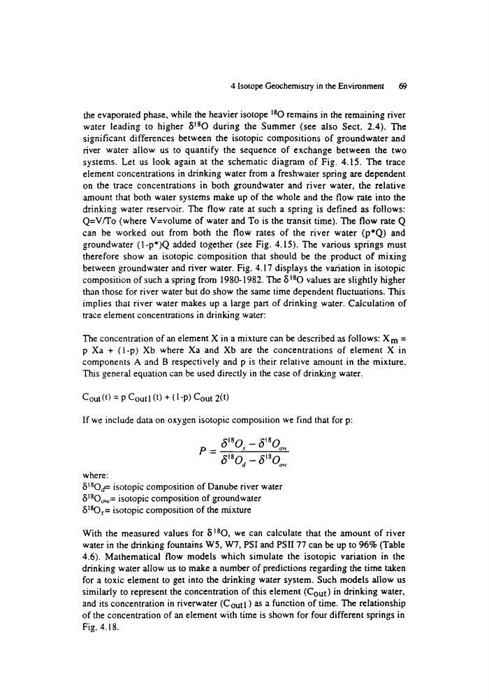
If we include data on oxygen isotopic composition we find that for p:
8o0,,
P = 61SO~_ ~8
5'80, - 6'SOo,,,
where:
5tSOd= isotopic composition of Danube river water
6tsOo,r= isotopic composition of groundwater
51sOt= isotopic composition of the mixture
With the measured values for 8~sO, we can calculate that the amount of river
water in the drinking fountains W5, W7, PSI and PSII 77 can be up to 96% (Table
4.6). Mathematical flow models which simulate the isotopic variation in the
drinking water allow us to make a number of predictions regarding the time taken
for a toxic element to get into the drinking water system. Such models allow us
similarly to represent the concentration of this element (Cout) in drinking water,
and its concentration in riverwater (Coutl) as a function of time. The relationship
of the concentration of an element with time is shown for four different springs in
Fig. 4.18.
69
the evaporated phase, while the heavier isotope 1sO remains in the remaining river
water leading to higher 5lso during the Summer (see also Sect. 2.4). The
significant differences between the isotopic compositions of groundwater and
river water allow us to quantify the sequence of exchange between the two
systems. Let us look again at the schematic diagram of Fig. 4.15. The trace
element concentrations in drinking water from a freshwater spring are dependent
on the trace concentrations in both groundwater and river water, the relative
amount that both water systems make up of the whole and the flow rate into the
drinking water reservoir. The flow rate at such a spring is defined as follows:
Q=VFFo (where V=volume of water and To is the transit time). The flow rate Q
can be worked out from both the flow rates of the river water ( p ' Q ) and
groundwater (l-p*)Q added together (see Fig. 4.15). The various springs must
therefore show an isotopic composition that should be the product of mixing
between groundwater and river water. Fig. 4.17 displays the variation in isotopic
composition of such a spring from 1980-1982. The 81sO values are slightly higher
than those for river water but do show the same time dependent fluctuations. This
implies that river water makes up a large part of drinking water. Calculation of
trace element concentrations in drinking water:
The concentration of an element X in a mixture can be described as follows: X m =
p Xa + (l-p) Xb where Xa and Xb are the concentrations of element X in
components A and B respectively and p is their relative amount in the mixture.
This general equation can be used directly in the case of drinking water.
Cout (t) = p Coutl (t) + (l-p) Cout 2(t)
If we include data on oxygen isotopic composition we find that for p:
8o0,,
P = 61SO~_ ~8
5'80, - 6'SOo,,,
where:
5tSOd= isotopic composition of Danube river water
6tsOo,r= isotopic composition of groundwater
51sOt= isotopic composition of the mixture
With the measured values for 8~sO, we can calculate that the amount of river
water in the drinking fountains W5, W7, PSI and PSII 77 can be up to 96% (Table
4.6). Mathematical flow models which simulate the isotopic variation in the
drinking water allow us to make a number of predictions regarding the time taken
for a toxic element to get into the drinking water system. Such models allow us
similarly to represent the concentration of this element (Cout) in drinking water,
and its concentration in riverwater (Coutl) as a function of time. The relationship
of the concentration of an element with time is shown for four different springs in
Fig. 4.18.