

79
the preceding half year still remain visible in a
depth between about 0.22 m and 0.35 m below the
sediment surface. Below a depth of 0.4 m no
further non-steady states can be seen, a constant
and steady-state mean concentration of ‘5.5’
prevails.
The conditions proposed in Figure 3.4
describe a very extreme situation. On the one
hand, the half-yearly alternating concentrations
differ by a whole order of magnitude, on the other
hand, no transitory periods with intermediate
concentrations were anticipated. Seasonal variations in nature usually display smaller concentration differences and are also likely to possess
transitory intermediate concentrations. Both
diminish the effects of non-steady state formation
in sedimentary depths as were shown in the
example of Figure 3.4.
Figure 3.4 also demonstrates clearly the
effects of the analytical precision on differentiating steady state and non-steady states in pore
water. In the theoretical calculation shown in
Figure 3.4, the difference between both curves is
still visible in form of a non-steady state at a
depth between 0.22 and 0.4 m. However, if the
possible errors are taken into consideration that
occur during sampling and in the analytic treatment of pore water samples (Sects. 3.3 - 3.5), then
there is likely to be no current parameter with
which these differences could be discovered
practically. Below a depth of 0.2 m, one would
always measure the same concentration and
consequently judge the situation as stationary, or
as a steady state.
3.2.2
The Steady State Situation
and Fick’s First Law of Diffusion
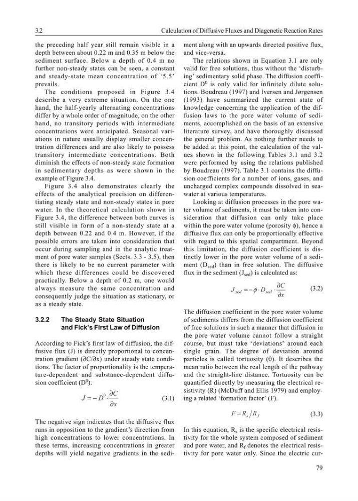
According to Fick’s first law of diffusion, the diffusive flux (J) is directly proportional to concentration gradient (∂C/∂x) under steady state conditions. The factor of proportionality is the temperature-dependent and substance-dependent diffusion coefficient (D 0 ):
J
D
C
x
= − ⋅
0 ∂
∂
(3.1)
The negative sign indicates that the diffusive flux
runs in opposition to the gradient’s direction from
high concentrations to lower concentrations. In
these terms, increasing concentrations in greater
depths will yield negative gradients in the sediment along with an upwards directed positive flux,
and vice-versa.
The relations shown in Equation 3.1 are only
valid for free solutions, thus without the ‘disturbing’ sedimentary solid phase. The diffusion coefficient D 0 is only valid for infinitely dilute solutions. Boudreau (1997) and Iversen and Jørgensen
(1993) have summarized the current state of
knowledge concerning the application of the diffusion laws to the pore water volume of sediments, accomplished on the basis of an extensive
literature survey, and have thoroughly discussed
the general problem. As nothing further needs to
be added at this point, the calculation of the values shown in the following Tables 3.1 and 3.2
were performed by using the relations published
by Boudreau (1997). Table 3.1 contains the diffusion coefficients for a number of ions, gases, and
uncharged complex compounds dissolved in seawater at various temperatures.
Looking at diffusion processes in the pore water volume of sediments, it must be taken into consideration that diffusion can only take place
within the pore water volume (porosity φ), hence a
diffusive flux can only be proportionally effective
with regard to this spatial compartment. Beyond
this limitation, the diffusion coefficient is distinctly lower in the pore water volume of a sediment (D sed ) than in free solution. The diffusive
flux in the sediment (J sed ) is calculated as:
x
C
D
J
sed
sed
∂
∂
⋅
⋅
−
= φ
(3.2)
The diffusion coefficient in the pore water volume
of sediments differs from the diffusion coefficient
of free solutions in such a manner that diffusion in
the pore water volume cannot follow a straight
course, but must take ‘deviations’ around each
single grain. The degree of deviation around
particles is called tortuosity (θ). It describes the
mean ratio between the real length of the pathway
and the straight-line distance. Tortuosity can be
quantified directly by measuring the electrical resistivity (R) (McDuff and Ellis 1979) and employing a related ‘formation factor’ (F).
f
s R
R
F =
(3.3)
In this equation, R s is the specific electrical resistivity for the whole system composed of sediment
and pore water, and R f denotes the electrical resistivity for pore water only. Since the electric cur3.2
Calculation of Diffusive Fluxes and Diagenetic Reaction Rates
the preceding half year still remain visible in a
depth between about 0.22 m and 0.35 m below the
sediment surface. Below a depth of 0.4 m no
further non-steady states can be seen, a constant
and steady-state mean concentration of ‘5.5’
prevails.
The conditions proposed in Figure 3.4
describe a very extreme situation. On the one
hand, the half-yearly alternating concentrations
differ by a whole order of magnitude, on the other
hand, no transitory periods with intermediate
concentrations were anticipated. Seasonal variations in nature usually display smaller concentration differences and are also likely to possess
transitory intermediate concentrations. Both
diminish the effects of non-steady state formation
in sedimentary depths as were shown in the
example of Figure 3.4.
Figure 3.4 also demonstrates clearly the
effects of the analytical precision on differentiating steady state and non-steady states in pore
water. In the theoretical calculation shown in
Figure 3.4, the difference between both curves is
still visible in form of a non-steady state at a
depth between 0.22 and 0.4 m. However, if the
possible errors are taken into consideration that
occur during sampling and in the analytic treatment of pore water samples (Sects. 3.3 - 3.5), then
there is likely to be no current parameter with
which these differences could be discovered
practically. Below a depth of 0.2 m, one would
always measure the same concentration and
consequently judge the situation as stationary, or
as a steady state.
3.2.2
The Steady State Situation
and Fick’s First Law of Diffusion
According to Fick’s first law of diffusion, the diffusive flux (J) is directly proportional to concentration gradient (∂C/∂x) under steady state conditions. The factor of proportionality is the temperature-dependent and substance-dependent diffusion coefficient (D 0 ):
J
D
C
x
= − ⋅
0 ∂
∂
(3.1)
The negative sign indicates that the diffusive flux
runs in opposition to the gradient’s direction from
high concentrations to lower concentrations. In
these terms, increasing concentrations in greater
depths will yield negative gradients in the sediment along with an upwards directed positive flux,
and vice-versa.
The relations shown in Equation 3.1 are only
valid for free solutions, thus without the ‘disturbing’ sedimentary solid phase. The diffusion coefficient D 0 is only valid for infinitely dilute solutions. Boudreau (1997) and Iversen and Jørgensen
(1993) have summarized the current state of
knowledge concerning the application of the diffusion laws to the pore water volume of sediments, accomplished on the basis of an extensive
literature survey, and have thoroughly discussed
the general problem. As nothing further needs to
be added at this point, the calculation of the values shown in the following Tables 3.1 and 3.2
were performed by using the relations published
by Boudreau (1997). Table 3.1 contains the diffusion coefficients for a number of ions, gases, and
uncharged complex compounds dissolved in seawater at various temperatures.
Looking at diffusion processes in the pore water volume of sediments, it must be taken into consideration that diffusion can only take place
within the pore water volume (porosity φ), hence a
diffusive flux can only be proportionally effective
with regard to this spatial compartment. Beyond
this limitation, the diffusion coefficient is distinctly lower in the pore water volume of a sediment (D sed ) than in free solution. The diffusive
flux in the sediment (J sed ) is calculated as:
x
C
D
J
sed
sed
∂
∂
⋅
⋅
−
= φ
(3.2)
The diffusion coefficient in the pore water volume
of sediments differs from the diffusion coefficient
of free solutions in such a manner that diffusion in
the pore water volume cannot follow a straight
course, but must take ‘deviations’ around each
single grain. The degree of deviation around
particles is called tortuosity (θ). It describes the
mean ratio between the real length of the pathway
and the straight-line distance. Tortuosity can be
quantified directly by measuring the electrical resistivity (R) (McDuff and Ellis 1979) and employing a related ‘formation factor’ (F).
f
s R
R
F =
(3.3)
In this equation, R s is the specific electrical resistivity for the whole system composed of sediment
and pore water, and R f denotes the electrical resistivity for pore water only. Since the electric cur3.2
Calculation of Diffusive Fluxes and Diagenetic Reaction Rates