

2
Physical Properties of Marine Sediments
38
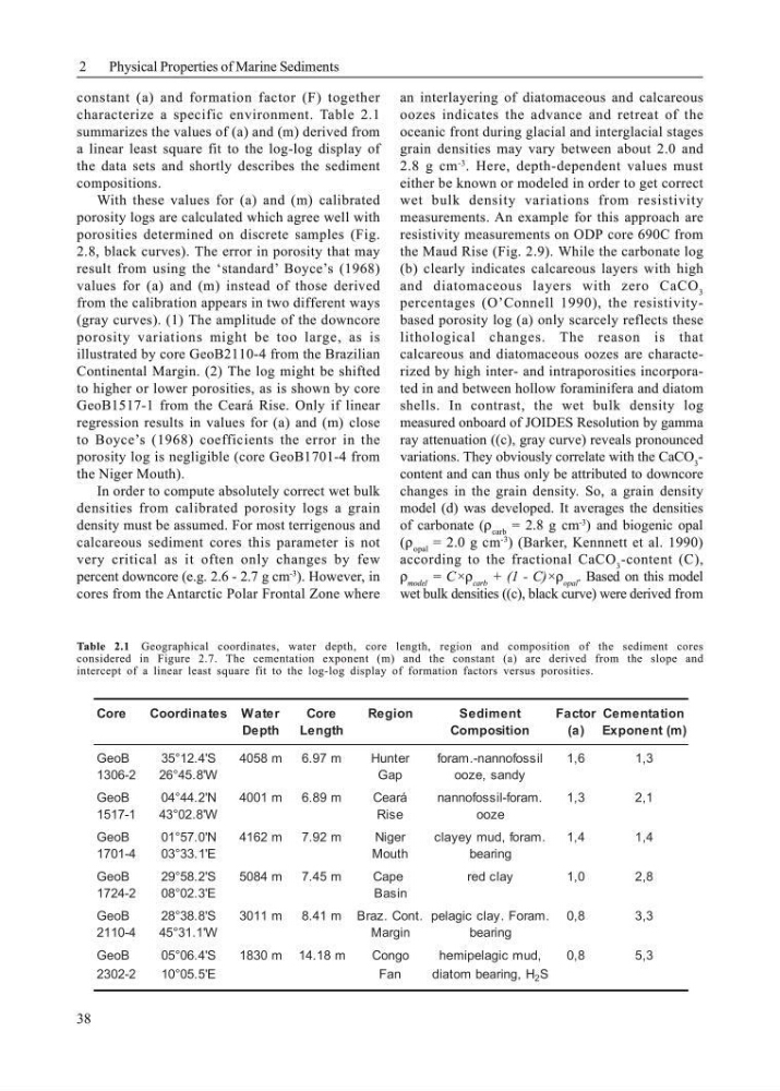
Table 2.1 Geographical coordinates, water depth, core length, region and composition of the sediment cores
considered in Figure 2.7. The cementation exponent (m) and the constant (a) are derived from the slope and
intercept of a linear least square fit to the log-log display of formation factors versus porosities.
constant (a) and formation factor (F) together
characterize a specific environment. Table 2.1
summarizes the values of (a) and (m) derived from
a linear least square fit to the log-log display of
the data sets and shortly describes the sediment
compositions.
With these values for (a) and (m) calibrated
porosity logs are calculated which agree well with
porosities determined on discrete samples (Fig.
2.8, black curves). The error in porosity that may
result from using the ‘standard’ Boyce’s (1968)
values for (a) and (m) instead of those derived
from the calibration appears in two different ways
(gray curves). (1) The amplitude of the downcore
porosity variations might be too large, as is
illustrated by core GeoB2110-4 from the Brazilian
Continental Margin. (2) The log might be shifted
to higher or lower porosities, as is shown by core
GeoB1517-1 from the Ceará Rise. Only if linear
regression results in values for (a) and (m) close
to Boyce’s (1968) coefficients the error in the
porosity log is negligible (core GeoB1701-4 from
the Niger Mouth).
In order to compute absolutely correct wet bulk
densities from calibrated porosity logs a grain
density must be assumed. For most terrigenous and
calcareous sediment cores this parameter is not
very critical as it often only changes by few
percent downcore (e.g. 2.6 - 2.7 g cm
-3
). However, in
cores from the Antarctic Polar Frontal Zone where
an interlayering of diatomaceous and calcareous
oozes indicates the advance and retreat of the
oceanic front during glacial and interglacial stages
grain densities may vary between about 2.0 and
2.8 g cm
-3
. Here, depth-dependent values must
either be known or modeled in order to get correct
wet bulk density variations from resistivity
measurements. An example for this approach are
resistivity measurements on ODP core 690C from
the Maud Rise (Fig. 2.9). While the carbonate log
(b) clearly indicates calcareous layers with high
and diatomaceous layers with zero CaCO 3
percentages (O’Connell 1990), the resistivitybased porosity log (a) only scarcely reflects these
lithological changes. The reason is that
calcareous and diatomaceous oozes are characterized by high inter- and intraporosities incorporated in and between hollow foraminifera and diatom
shells. In contrast, the wet bulk density log
measured onboard of JOIDES Resolution by gamma
ray attenuation ((c), gray curve) reveals pronounced
variations. They obviously correlate with the CaCO 3 -
content and can thus only be attributed to downcore
changes in the grain density. So, a grain density
model (d) was developed. It averages the densities
of carbonate (ρ carb = 2.8 g cm
-3
) and biogenic opal
(ρ opal = 2.0 g cm
-3
) (Barker, Kennnett et al. 1990)
according to the fractional CaCO 3 -content (C),
ρ model = C×ρ carb + (1 - C)×ρ opal . Based on this model
wet bulk densities ((c), black curve) were derived from
Core
Coordinates Water
Core
Region
Sediment
Factor Cementation
Depth
Length
Composition
(a) Exponent (m)
GeoB
35°12.4'S
4058 m
6.97 m
Hunter
foram.-nannofossil
1,6
1,3
1306-2
26°45.8'W
Gap
ooze, sandy
GeoB
04°44.2'N
4001 m
6.89 m
Ceará
nannofossil-foram.
1,3
2,1
1517-1
43°02.8'W
Rise
ooze
GeoB
01°57.0'N
4162 m
7.92 m
Niger
clayey mud, foram.
1,4
1,4
1701-4
03°33.1'E
Mouth
bearing
GeoB
29°58.2'S
5084 m
7.45 m
Cape
red clay
1,0
2,8
1724-2
08°02.3'E
Basin
GeoB
28°38.8'S
3011 m
8.41 m Braz. Cont. pelagic clay. Foram. 0,8
3,3
2110-4
45°31.1'W
Margin
bearing
GeoB
05°06.4'S
1830 m 14.18 m
Congo
hemipelagic mud,
0,8
5,3
2302-2
10°05.5'E
Fan
diatom bearing, H 2 S
Physical Properties of Marine Sediments
38
Table 2.1 Geographical coordinates, water depth, core length, region and composition of the sediment cores
considered in Figure 2.7. The cementation exponent (m) and the constant (a) are derived from the slope and
intercept of a linear least square fit to the log-log display of formation factors versus porosities.
constant (a) and formation factor (F) together
characterize a specific environment. Table 2.1
summarizes the values of (a) and (m) derived from
a linear least square fit to the log-log display of
the data sets and shortly describes the sediment
compositions.
With these values for (a) and (m) calibrated
porosity logs are calculated which agree well with
porosities determined on discrete samples (Fig.
2.8, black curves). The error in porosity that may
result from using the ‘standard’ Boyce’s (1968)
values for (a) and (m) instead of those derived
from the calibration appears in two different ways
(gray curves). (1) The amplitude of the downcore
porosity variations might be too large, as is
illustrated by core GeoB2110-4 from the Brazilian
Continental Margin. (2) The log might be shifted
to higher or lower porosities, as is shown by core
GeoB1517-1 from the Ceará Rise. Only if linear
regression results in values for (a) and (m) close
to Boyce’s (1968) coefficients the error in the
porosity log is negligible (core GeoB1701-4 from
the Niger Mouth).
In order to compute absolutely correct wet bulk
densities from calibrated porosity logs a grain
density must be assumed. For most terrigenous and
calcareous sediment cores this parameter is not
very critical as it often only changes by few
percent downcore (e.g. 2.6 - 2.7 g cm
-3
). However, in
cores from the Antarctic Polar Frontal Zone where
an interlayering of diatomaceous and calcareous
oozes indicates the advance and retreat of the
oceanic front during glacial and interglacial stages
grain densities may vary between about 2.0 and
2.8 g cm
-3
. Here, depth-dependent values must
either be known or modeled in order to get correct
wet bulk density variations from resistivity
measurements. An example for this approach are
resistivity measurements on ODP core 690C from
the Maud Rise (Fig. 2.9). While the carbonate log
(b) clearly indicates calcareous layers with high
and diatomaceous layers with zero CaCO 3
percentages (O’Connell 1990), the resistivitybased porosity log (a) only scarcely reflects these
lithological changes. The reason is that
calcareous and diatomaceous oozes are characterized by high inter- and intraporosities incorporated in and between hollow foraminifera and diatom
shells. In contrast, the wet bulk density log
measured onboard of JOIDES Resolution by gamma
ray attenuation ((c), gray curve) reveals pronounced
variations. They obviously correlate with the CaCO 3 -
content and can thus only be attributed to downcore
changes in the grain density. So, a grain density
model (d) was developed. It averages the densities
of carbonate (ρ carb = 2.8 g cm
-3
) and biogenic opal
(ρ opal = 2.0 g cm
-3
) (Barker, Kennnett et al. 1990)
according to the fractional CaCO 3 -content (C),
ρ model = C×ρ carb + (1 - C)×ρ opal . Based on this model
wet bulk densities ((c), black curve) were derived from
Core
Coordinates Water
Core
Region
Sediment
Factor Cementation
Depth
Length
Composition
(a) Exponent (m)
GeoB
35°12.4'S
4058 m
6.97 m
Hunter
foram.-nannofossil
1,6
1,3
1306-2
26°45.8'W
Gap
ooze, sandy
GeoB
04°44.2'N
4001 m
6.89 m
Ceará
nannofossil-foram.
1,3
2,1
1517-1
43°02.8'W
Rise
ooze
GeoB
01°57.0'N
4162 m
7.92 m
Niger
clayey mud, foram.
1,4
1,4
1701-4
03°33.1'E
Mouth
bearing
GeoB
29°58.2'S
5084 m
7.45 m
Cape
red clay
1,0
2,8
1724-2
08°02.3'E
Basin
GeoB
28°38.8'S
3011 m
8.41 m Braz. Cont. pelagic clay. Foram. 0,8
3,3
2110-4
45°31.1'W
Margin
bearing
GeoB
05°06.4'S
1830 m 14.18 m
Congo
hemipelagic mud,
0,8
5,3
2302-2
10°05.5'E
Fan
diatom bearing, H 2 S