

15 Conceptual Models and Computer Models
514
become completely forgotten by now. Afterwards
a FORTRAN version had followed (WATEQF)
released by Plummer et al. (1976) as well as
another revised version (WATEQ4F) by Ball and
Nordstrom (1991).
All these programs share the common feature
that they start out from water analyses which were
designed as comprehensive as possible, along
with conceiving the measured values as cumulative parameters (sums of all aquatic species),
only to subsequently allocate them to the various
aquatic species. This was done by applying
iteration calculus that accounts for the equilibria
related to the various aquatic species.
For instance, the measured value of calcium in
an ocean water sample containing 10.6 mmoles/l is
allocated to 9.51 mmol/l Ca
2+
, 1.08 mmol/l CaSO 4
0
,
0.04 mmol/l CaHCO 3
+
, and to a series of low
concentrated other calcium species in solution.
The analysis of sulfate yielding 29.26 mmol/l is
allocated accordingly to 14.67 mmol/l SO 4
2, 7.30
mmol/l NaSO 4
-
, 1.08 mmol/l CaSO 4
0
, 0.16 mmol/l
KSO 4
-
, and, likewise, to a number of low concentrated sulfate species. The procedure is similarly
applied to all analytical values. Table 15.2 summarizes the species allocations for the ocean water
analysis previously shown in Table 15.1.
Based on the activities of the non-complex
aquatic species (e.g. [Ca
2+
] or [SO 4
2], the next step
consists in calculating the saturation indices (SI)
of each compound mineral:
⎟
⎠
⎞
⎜
⎝
⎛
=
sp
K
IAP
SI log
(15.1)
In this equation IAP denotes the Ion Activity
Product (in the example of gypsum or anhydrite
these would be ([Ca
2+
]·[SO 4
2]). K SP is the solubility product constant of the respective mineral.
A saturation index SI = 0 describes the condition
in which the solution of the corresponding
mineral is just saturated, SI > 0 describes the
condition of supersaturation of the solution, SI <
0 its undersaturation. The activity [A] of a substance is calculated according to the equation:
A
A
A
γ
⋅
= )
(
]
[
(15.2)
Here, (A) is the concentration of a substance
measured in moles/l and γ A is the activity coefficient calculated as a function of the overall
ionic strength in the solution. For infinitesimal
diluted solutions, the activity coefficients assume the value of 1; hence, activity equals
concentration. In ocean water, the various monovalent ions, or ion pairs, display activity
coefficients somewhere around 0.75; whereas
the various divalent ions, or ion pairs, display
values around 0.2 (cf. Table 15.2, last column).
After transformation, the equation 15.1 to calculate the saturation index of the mineral gypsum
reads:
⎟
⎟
⎠
⎞
⎜
⎜
⎝
⎛
⋅
=
−
+
gypsum
sp
gypsum
K
SO
Ca
SI
,
2
4
2
]
[
]
[
log
(15.3)
If we now insert the solubility product constant
for gypsum K sp , gypsum = 2.63·10 -5 in the equation
and the exemplary values mentioned above for
ocean water (activity coefficients of divalent ions
≈ 0.2; concentration of Ca 2+ = 9.15/1000 mol/l;
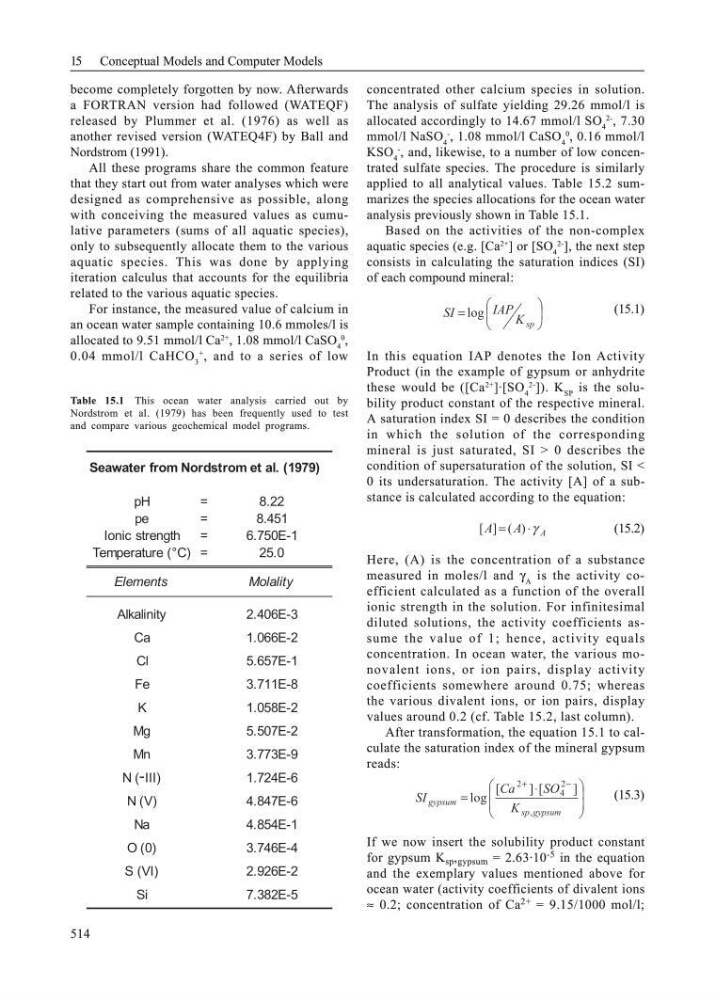
Table 15.1 This ocean water analysis carried out by
Nordstrom et al. (1979) has been frequently used to test
and compare various geochemical model programs.
Seawater from Nordstrom et al. (1979)
pH
=
8.22
pe
=
8.451
Ionic strength =
6.750E-1
Temperature (°C) =
25.0
Elements
Molality
Alkalinity
2.406E-3
Ca
1.066E-2
Cl
5.657E-1
Fe
3.711E-8
K
1.058E-2
Mg
5.507E-2
Mn
3.773E-9
N (-III)
1.724E-6
N (V)
4.847E-6
Na
4.854E-1
O (0)
3.746E-4
S (VI)
2.926E-2
Si
7.382E-5
514
become completely forgotten by now. Afterwards
a FORTRAN version had followed (WATEQF)
released by Plummer et al. (1976) as well as
another revised version (WATEQ4F) by Ball and
Nordstrom (1991).
All these programs share the common feature
that they start out from water analyses which were
designed as comprehensive as possible, along
with conceiving the measured values as cumulative parameters (sums of all aquatic species),
only to subsequently allocate them to the various
aquatic species. This was done by applying
iteration calculus that accounts for the equilibria
related to the various aquatic species.
For instance, the measured value of calcium in
an ocean water sample containing 10.6 mmoles/l is
allocated to 9.51 mmol/l Ca
2+
, 1.08 mmol/l CaSO 4
0
,
0.04 mmol/l CaHCO 3
+
, and to a series of low
concentrated other calcium species in solution.
The analysis of sulfate yielding 29.26 mmol/l is
allocated accordingly to 14.67 mmol/l SO 4
2, 7.30
mmol/l NaSO 4
-
, 1.08 mmol/l CaSO 4
0
, 0.16 mmol/l
KSO 4
-
, and, likewise, to a number of low concentrated sulfate species. The procedure is similarly
applied to all analytical values. Table 15.2 summarizes the species allocations for the ocean water
analysis previously shown in Table 15.1.
Based on the activities of the non-complex
aquatic species (e.g. [Ca
2+
] or [SO 4
2], the next step
consists in calculating the saturation indices (SI)
of each compound mineral:
⎟
⎠
⎞
⎜
⎝
⎛
=
sp
K
IAP
SI log
(15.1)
In this equation IAP denotes the Ion Activity
Product (in the example of gypsum or anhydrite
these would be ([Ca
2+
]·[SO 4
2]). K SP is the solubility product constant of the respective mineral.
A saturation index SI = 0 describes the condition
in which the solution of the corresponding
mineral is just saturated, SI > 0 describes the
condition of supersaturation of the solution, SI <
0 its undersaturation. The activity [A] of a substance is calculated according to the equation:
A
A
A
γ
⋅
= )
(
]
[
(15.2)
Here, (A) is the concentration of a substance
measured in moles/l and γ A is the activity coefficient calculated as a function of the overall
ionic strength in the solution. For infinitesimal
diluted solutions, the activity coefficients assume the value of 1; hence, activity equals
concentration. In ocean water, the various monovalent ions, or ion pairs, display activity
coefficients somewhere around 0.75; whereas
the various divalent ions, or ion pairs, display
values around 0.2 (cf. Table 15.2, last column).
After transformation, the equation 15.1 to calculate the saturation index of the mineral gypsum
reads:
⎟
⎟
⎠
⎞
⎜
⎜
⎝
⎛
⋅
=
−
+
gypsum
sp
gypsum
K
SO
Ca
SI
,
2
4
2
]
[
]
[
log
(15.3)
If we now insert the solubility product constant
for gypsum K sp , gypsum = 2.63·10 -5 in the equation
and the exemplary values mentioned above for
ocean water (activity coefficients of divalent ions
≈ 0.2; concentration of Ca 2+ = 9.15/1000 mol/l;
Table 15.1 This ocean water analysis carried out by
Nordstrom et al. (1979) has been frequently used to test
and compare various geochemical model programs.
Seawater from Nordstrom et al. (1979)
pH
=
8.22
pe
=
8.451
Ionic strength =
6.750E-1
Temperature (°C) =
25.0
Elements
Molality
Alkalinity
2.406E-3
Ca
1.066E-2
Cl
5.657E-1
Fe
3.711E-8
K
1.058E-2
Mg
5.507E-2
Mn
3.773E-9
N (-III)
1.724E-6
N (V)
4.847E-6
Na
4.854E-1
O (0)
3.746E-4
S (VI)
2.926E-2
Si
7.382E-5