

290
Chapter 15: Multivariate Statistical Modeling:
matrix as a function of 1 in this general formulation. However, Wa11ace and
Dickinson (1972) pointed out the possibility of studying the cross-spectrum
matrix at an infinitesimal frequency interval around 10' They suggested investigating the eigenstructure of (15.18) averaged over the frequency interval
10 ± f in analogy to an EOF analysis. The complex eigenvectors of this Hermitian matrix are ca11ed Complex EOFs. In analogy to 1-dimensional waves
which can be described by a complex function, one can derive the amplitude
and spatial phase relationship of an rn-dimensional wave from the complex
EOFs. Another way to interpret a complex EOF is to use the notion that the
cross-spectrum matrix of X at a positive frequency is also the cross-spectrum
matrix of Y. The eigenvectors of the latter can be interpreted according to
the definition ofY (15.20) which shows that the real and imaginary part ofY
are coherent with a fixed temporal phase shift of 90 0 at each frequency. This
suggests that if the real part of the complex EOF represents spatial structure at frequency I, the imaginary part represents then the spatial structure
at the same frequency but with a time lag of one quarter of the oscillation
period T = 1/1. The Wallace and Dickinson approach is denoted hereafter
as complex EOF analysis in the Irequency domain.
The filtered time series of Y in which a11 spectral components outside the
-'
frequency interval 10 ± f are removed is denoted by Y . The cross-spectrum
matrixofY averaged over the infinitesimal frequency interval lo±f is also the
-'
cross-spectrum matrix of Y . Furthermore, since the cross-spectrum matrix
ry, is the Fourier transform of cross-covariance matrix Ey' at frequency I,
one has'
00
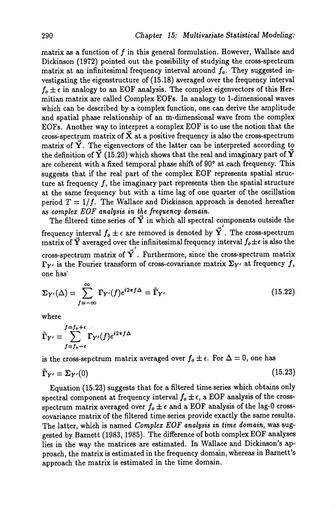
Ey,(~) = E rY'(f)e i2 '1r 1 ll. = ry,
(15.22)
1=-00
where
1=lo+f
-
'"'"
'2 1 ll.
ry, = L.J ry'(f)e' 'Ir
1=lo-f
is the cross-sepctrum matrix averaged over 10 ± f. For ~ = 0, one has
(15.23)
Equation (15.23) suggests that for a filtered time series which obtains only
spectral component at frequency interval 10 ± f, a EOF analysis of the crossspectrum matrix averaged over 10 ± fand a EOF analysis of the lag-O crosscovariance matrix of the filtered time series provide exact1y the same results.
The latter, which is named Complex EOF analysis in time domain, was suggested by Barnett (1983, 1985). The difference ofboth complex EOF analyses
lies in the way the matrices are estimated, In Wa11ace and Dickinson's approach, the matrix is estimated in the frequency domain, whereas in Barnett's
approach the matrix is estimated in the time domain.
Chapter 15: Multivariate Statistical Modeling:
matrix as a function of 1 in this general formulation. However, Wa11ace and
Dickinson (1972) pointed out the possibility of studying the cross-spectrum
matrix at an infinitesimal frequency interval around 10' They suggested investigating the eigenstructure of (15.18) averaged over the frequency interval
10 ± f in analogy to an EOF analysis. The complex eigenvectors of this Hermitian matrix are ca11ed Complex EOFs. In analogy to 1-dimensional waves
which can be described by a complex function, one can derive the amplitude
and spatial phase relationship of an rn-dimensional wave from the complex
EOFs. Another way to interpret a complex EOF is to use the notion that the
cross-spectrum matrix of X at a positive frequency is also the cross-spectrum
matrix of Y. The eigenvectors of the latter can be interpreted according to
the definition ofY (15.20) which shows that the real and imaginary part ofY
are coherent with a fixed temporal phase shift of 90 0 at each frequency. This
suggests that if the real part of the complex EOF represents spatial structure at frequency I, the imaginary part represents then the spatial structure
at the same frequency but with a time lag of one quarter of the oscillation
period T = 1/1. The Wallace and Dickinson approach is denoted hereafter
as complex EOF analysis in the Irequency domain.
The filtered time series of Y in which a11 spectral components outside the
-'
frequency interval 10 ± f are removed is denoted by Y . The cross-spectrum
matrixofY averaged over the infinitesimal frequency interval lo±f is also the
-'
cross-spectrum matrix of Y . Furthermore, since the cross-spectrum matrix
ry, is the Fourier transform of cross-covariance matrix Ey' at frequency I,
one has'
00
Ey,(~) = E rY'(f)e i2 '1r 1 ll. = ry,
(15.22)
1=-00
where
1=lo+f
-
'"'"
'2 1 ll.
ry, = L.J ry'(f)e' 'Ir
1=lo-f
is the cross-sepctrum matrix averaged over 10 ± f. For ~ = 0, one has
(15.23)
Equation (15.23) suggests that for a filtered time series which obtains only
spectral component at frequency interval 10 ± f, a EOF analysis of the crossspectrum matrix averaged over 10 ± fand a EOF analysis of the lag-O crosscovariance matrix of the filtered time series provide exact1y the same results.
The latter, which is named Complex EOF analysis in time domain, was suggested by Barnett (1983, 1985). The difference ofboth complex EOF analyses
lies in the way the matrices are estimated, In Wa11ace and Dickinson's approach, the matrix is estimated in the frequency domain, whereas in Barnett's
approach the matrix is estimated in the time domain.