

Section 13.4: Canonical Correlation Analysis
249
values< -2. Together with the information provided by the patterns (Figure
13.3) such large negative coefficients represent extremely cold winters, such
as 1940 and 1941, with mean negative anomalies of the order of< -4K. The
distribution of the first EOF coefficient is markedly skewed (Figure 13.5)
whereas the distribution of the second coefficient is fairly symmetrie. The
time series of the 2nd coefficient, depicted in Figure 13.4 shows no dramatic
outliers but, interestingly, an upward trend translates at the stations with
a slow warming of the Alpine region (~ 0.005Kjyr) and a gradual cooling
(~ 0.01Kjyr) in the lowlands.
This is about all that the EOFs can tell us about the evolution of winter
mean temperature in Central Europe in the years 1901-80. We will come
back to this example in Section 13.4.4.
13.4 Canonical Correlation Analysis
We assume for this section again that the expectations of the considered
random vectors X and Y vanish: iix = iiy = O.
13.4.1 Definition of Canonical Correlation Patterns
In the Canonical Correlation Analysis [CCA, proposed by Hotelling (1936)
and introduced into climate research by, among others, Barnett and Preisendorfer (1987)] not one random vector X is expanded into a finite set of
vectors but a pair of two simultaneously observed vectors X and Y:
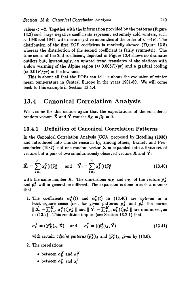
K
~
~
Y
~k
and Y t = L...J CXk (t)py
(13.40)
k=l
with the same number K. The dimensions mx and my of the vectors P1
and P';' will in general be different. The expansion is done in such a manner
that
1. The coefficients cxf (t) and cxr (t) in (13.40) are optimal in a
least square sense [i.e., for given patterns p'! and p;' the norms
11 Xt - 2:::=1 cxf (t)p! 11 and 11 Y t - 2:::=1 cxr (t)p;' 11 are minimized, as
in (13.2)]. This condition implies (see Section 13.2.1) that
(13.41)
with certain adjoint patterns (Pi)A and (P{;)A given by (13.6).
2. The correlations
• between cxf and cxf
• between cxr and cxr
249
values< -2. Together with the information provided by the patterns (Figure
13.3) such large negative coefficients represent extremely cold winters, such
as 1940 and 1941, with mean negative anomalies of the order of< -4K. The
distribution of the first EOF coefficient is markedly skewed (Figure 13.5)
whereas the distribution of the second coefficient is fairly symmetrie. The
time series of the 2nd coefficient, depicted in Figure 13.4 shows no dramatic
outliers but, interestingly, an upward trend translates at the stations with
a slow warming of the Alpine region (~ 0.005Kjyr) and a gradual cooling
(~ 0.01Kjyr) in the lowlands.
This is about all that the EOFs can tell us about the evolution of winter
mean temperature in Central Europe in the years 1901-80. We will come
back to this example in Section 13.4.4.
13.4 Canonical Correlation Analysis
We assume for this section again that the expectations of the considered
random vectors X and Y vanish: iix = iiy = O.
13.4.1 Definition of Canonical Correlation Patterns
In the Canonical Correlation Analysis [CCA, proposed by Hotelling (1936)
and introduced into climate research by, among others, Barnett and Preisendorfer (1987)] not one random vector X is expanded into a finite set of
vectors but a pair of two simultaneously observed vectors X and Y:
K
~
~
Y
~k
and Y t = L...J CXk (t)py
(13.40)
k=l
with the same number K. The dimensions mx and my of the vectors P1
and P';' will in general be different. The expansion is done in such a manner
that
1. The coefficients cxf (t) and cxr (t) in (13.40) are optimal in a
least square sense [i.e., for given patterns p'! and p;' the norms
11 Xt - 2:::=1 cxf (t)p! 11 and 11 Y t - 2:::=1 cxr (t)p;' 11 are minimized, as
in (13.2)]. This condition implies (see Section 13.2.1) that
(13.41)
with certain adjoint patterns (Pi)A and (P{;)A given by (13.6).
2. The correlations
• between cxf and cxf
• between cxr and cxr