

152
Chapter 8: Statistical Analysis of GCM Output
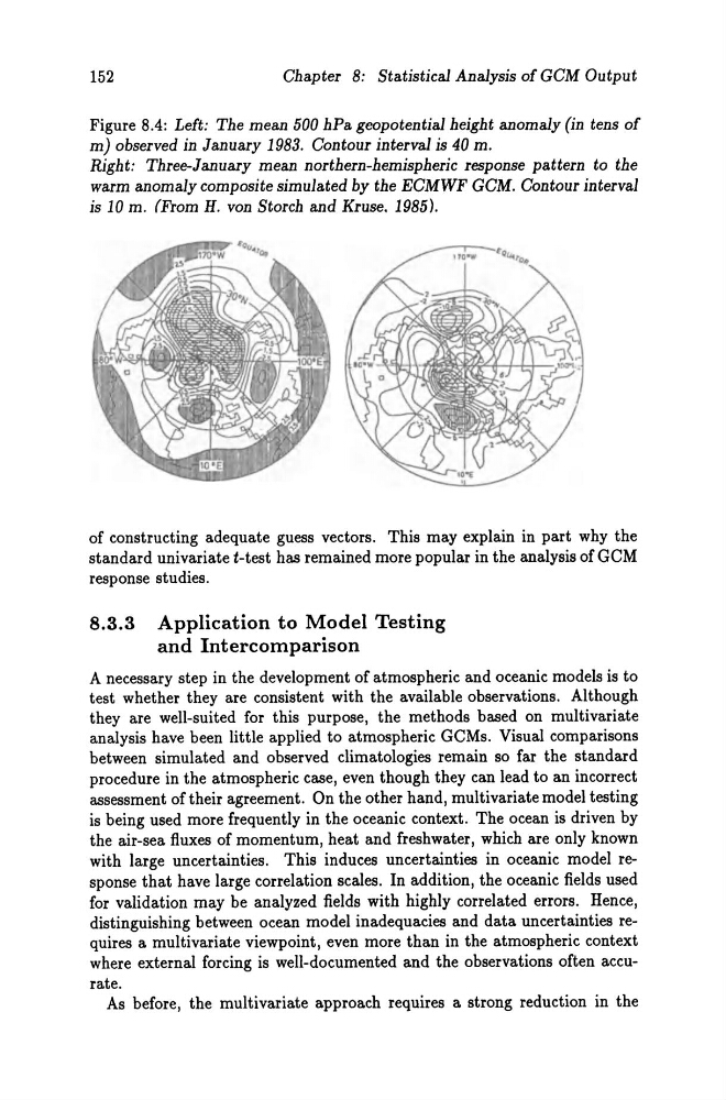
Figure 8.4: Left: The mean 500 hPa geopotential height anomaly (in tens of
m) observed in January 1983. Contour interval is 40 m.
Right: Three-January mean northern-hemispheric response pattern to the
warm anomaly composite simulated by the ECMWF GCM. Contour interval
is 10 m. (From H. von Storch and Kruse. 1985).
of constructing adequate guess vectors. This may explain in part why the
standard univariate t-test has remained more popular in the analysis of GCM
response studies.
8.3.3 Application to Model Testing
and Intercomparison
A necessary step in the development of atmospheric and oceanic models is to
test whether they are consistent with the available observations. Although
they are well-suited for this purpose, the methods based on multivariate
analysis have been little applied to atmospheric GCMs. Visual comparisons
between simulated and observed climatologies remain so far the standard
procedure in the atmospheric case, even though they can lead to an incorrect
assessment of their agreement. On the other hand, multivariate model testing
is being used more frequently in the oceanic context. The ocean is driven by
the air-sea fluxes of moment um, heat and freshwater, which are only known
with large uncertainties. This induces uncertainties in oceanic model response that have large correlation scales. In addition, the oceanic fields used
for validation may be analyzed fields with highly correlated errors. Hence,
distinguishing between ocean model inadequacies and data uncertainties requires a multivariate viewpoint, even more than in the atmospheric context
where extern al forcing is well-documented and the observations often accurate.
As before, the multivariate approach requires a strong reduction in the
Chapter 8: Statistical Analysis of GCM Output
Figure 8.4: Left: The mean 500 hPa geopotential height anomaly (in tens of
m) observed in January 1983. Contour interval is 40 m.
Right: Three-January mean northern-hemispheric response pattern to the
warm anomaly composite simulated by the ECMWF GCM. Contour interval
is 10 m. (From H. von Storch and Kruse. 1985).
of constructing adequate guess vectors. This may explain in part why the
standard univariate t-test has remained more popular in the analysis of GCM
response studies.
8.3.3 Application to Model Testing
and Intercomparison
A necessary step in the development of atmospheric and oceanic models is to
test whether they are consistent with the available observations. Although
they are well-suited for this purpose, the methods based on multivariate
analysis have been little applied to atmospheric GCMs. Visual comparisons
between simulated and observed climatologies remain so far the standard
procedure in the atmospheric case, even though they can lead to an incorrect
assessment of their agreement. On the other hand, multivariate model testing
is being used more frequently in the oceanic context. The ocean is driven by
the air-sea fluxes of moment um, heat and freshwater, which are only known
with large uncertainties. This induces uncertainties in oceanic model response that have large correlation scales. In addition, the oceanic fields used
for validation may be analyzed fields with highly correlated errors. Hence,
distinguishing between ocean model inadequacies and data uncertainties requires a multivariate viewpoint, even more than in the atmospheric context
where extern al forcing is well-documented and the observations often accurate.
As before, the multivariate approach requires a strong reduction in the