

102
Chapter 6: Analysing the Boreal Summer Relationship
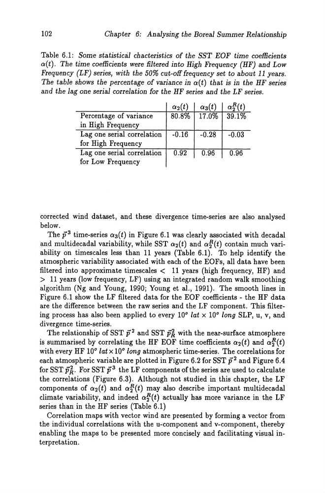
Table 6.1: Some statistical chacteristics of the SST EOF time coefflcients
a(t). The time coefflcients were fiItered into High Frequency (HF) and Low
Frequency (LF) series, with the 50% cut-off frequency set to about 11 years.
The table shows the percentage of variance in a(t) that is in the HF series
and the lag one serial correlation for the HF series and the LF series.
a2(t) a3(t) af(t)
Percentage of variance
80.8% 17.0% 39.1%
in High Frequency
Lag one serial correlation -0.16
-0.28
-0.03
for High Frequency
Lag one serial correlation
0.92
0.96
0.96
for Low Frequency
corrected wind dataset, and these divergence time-series are also analysed
below.
The p 3 time-series a3(t) in Figure 6.1 was clearly associated with decadal
and multidecadal variability, while SST a2(t) and ar(t) contain much variability on timescales less than 11 years (Table 6.1). To help identify the
atmospheric variability associated with each of the EOFs, all data have been
filtered into approximate timescales < 11 years (high frequency, HF) and
> 11 years (low frequency, LF) using an integrated random walk smoothing
algorithm (Ng and Young, 1990; Young et al., 1991). The smooth lines in
Figure 6.1 show the LF filtered data for the EOF coefficients - the HF data
are the difference between the raw series and the LF component. This filtering process has also been applied to every 10° lat x 10° lang SLP, u, v, and
divergence time-series.
The relationship of SST p2 and SST PA with the near-surface atmosphere
is summarised by correlating the HF EOF time coefficients a2(t) and af(t)
with every HF 10° lat x 10° lang atmospheric time-series. The correlations for
each atmospheric variable are plotted in Figure 6.2 for SST p2 and Figure 6.4
for SST p'k For SST p3 the LF components ofthe series are used to calculate
the correlations (Figure 6.3). Although not studied in this chapter, the LF
components of a2(t) and af(t) mayaiso describe important multidecadal
climate variability, and indeed ar(t) actually has more variance in the LF
se ries than in the HF series (Table 6.1)
Correlation maps with vector wind are presented by forming a vector from
the individual correlations with the u-component and v-component, thereby
enabling the maps to be presented more concisely and facilitating visual interpretation.
Chapter 6: Analysing the Boreal Summer Relationship
Table 6.1: Some statistical chacteristics of the SST EOF time coefflcients
a(t). The time coefflcients were fiItered into High Frequency (HF) and Low
Frequency (LF) series, with the 50% cut-off frequency set to about 11 years.
The table shows the percentage of variance in a(t) that is in the HF series
and the lag one serial correlation for the HF series and the LF series.
a2(t) a3(t) af(t)
Percentage of variance
80.8% 17.0% 39.1%
in High Frequency
Lag one serial correlation -0.16
-0.28
-0.03
for High Frequency
Lag one serial correlation
0.92
0.96
0.96
for Low Frequency
corrected wind dataset, and these divergence time-series are also analysed
below.
The p 3 time-series a3(t) in Figure 6.1 was clearly associated with decadal
and multidecadal variability, while SST a2(t) and ar(t) contain much variability on timescales less than 11 years (Table 6.1). To help identify the
atmospheric variability associated with each of the EOFs, all data have been
filtered into approximate timescales < 11 years (high frequency, HF) and
> 11 years (low frequency, LF) using an integrated random walk smoothing
algorithm (Ng and Young, 1990; Young et al., 1991). The smooth lines in
Figure 6.1 show the LF filtered data for the EOF coefficients - the HF data
are the difference between the raw series and the LF component. This filtering process has also been applied to every 10° lat x 10° lang SLP, u, v, and
divergence time-series.
The relationship of SST p2 and SST PA with the near-surface atmosphere
is summarised by correlating the HF EOF time coefficients a2(t) and af(t)
with every HF 10° lat x 10° lang atmospheric time-series. The correlations for
each atmospheric variable are plotted in Figure 6.2 for SST p2 and Figure 6.4
for SST p'k For SST p3 the LF components ofthe series are used to calculate
the correlations (Figure 6.3). Although not studied in this chapter, the LF
components of a2(t) and af(t) mayaiso describe important multidecadal
climate variability, and indeed ar(t) actually has more variance in the LF
se ries than in the HF series (Table 6.1)
Correlation maps with vector wind are presented by forming a vector from
the individual correlations with the u-component and v-component, thereby
enabling the maps to be presented more concisely and facilitating visual interpretation.