

70
J.D. Albertson, G. Kiely and M.B. Parlange
3.1.6 Inertial range methods of determining dissipation rates
We review three methods for determining dissipation rates from inertial subrange scaling in the
spirit of Kolmogorov (1941): power spectra, second order structure functions, and third order
structure functions.
Spectral method
The dissipation rates (E and EO) have been determined most frequently from the one-dimensional
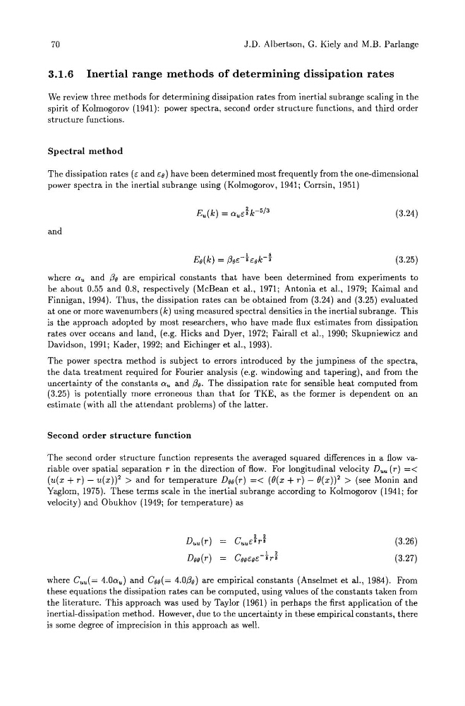
power spectra in the inertial sub range using (Kolmogorov, 1941; Corrsin, 1951)
(3.24 )
and
(3.25)
where au and Po are empirical constants that have been determined from experiments to
be about 0.55 and 0.8, respectively (McBean et al., 1971; Antonia et al., 1979; Kaimal and
Finnigan, 1994). Thus, the dissipation rates can be obtained from (3.24) and (3.25) evaluated
at one or more wavenumbers (k) using measured spectral densities in the inertial subrange. This
is the approach adopted by most researchers, who have made flux estimates from dissipation
rates over oceans and land, (e.g. Hicks and Dyer, 1972; Fairall et al., 1990; Skupniewicz and
Davidson, 1991; Kader, 1992; and Eichinger et al., 1993).
The power spectra method is subject to errors introduced by the jumpiness of the spectra,
the data treatment required for Fourier analysis (e.g. windowing and tapering), and from the
uncertainty of the constants au and 130. The dissipation rate for sensible heat computed from
(3.25) is potentially more erroneous than that for TKE, as the former is dependent on an
estimate (with all the attendant problems) of the latter.
Second order structure function
The second order structure function represents the averaged squared differences in a flow variable over spatial separation r in the direction of flow. For longitudinal velocity Duu (r) =<
(u(x + r) - U(X))2 > and for temperature Doo(r) =< (O(x + r) - O(x))2 > (see Monin and
Yaglom, 1975). These terms scale in the inertial subrange according to Kolmogorov (1941; for
velocity) and Obukhov (1949; for temperature) as
GuuE~r~
GOoEoE-~r~
(3.26)
(3.27)
where Guu (= 4.0au ) and Goo(= 4.0130) are empirical constants (Anselmet et al., 1984). From
these equations the dissipation rates can be computed, using values of the constants taken from
the literature. This approach was used by Taylor (1961) in perhaps the first application of the
inertial-dissipation method. However, due to the uncertainty in these empirical constants, there
is some degree of imprecision in this approach as well.
J.D. Albertson, G. Kiely and M.B. Parlange
3.1.6 Inertial range methods of determining dissipation rates
We review three methods for determining dissipation rates from inertial subrange scaling in the
spirit of Kolmogorov (1941): power spectra, second order structure functions, and third order
structure functions.
Spectral method
The dissipation rates (E and EO) have been determined most frequently from the one-dimensional
power spectra in the inertial sub range using (Kolmogorov, 1941; Corrsin, 1951)
(3.24 )
and
(3.25)
where au and Po are empirical constants that have been determined from experiments to
be about 0.55 and 0.8, respectively (McBean et al., 1971; Antonia et al., 1979; Kaimal and
Finnigan, 1994). Thus, the dissipation rates can be obtained from (3.24) and (3.25) evaluated
at one or more wavenumbers (k) using measured spectral densities in the inertial subrange. This
is the approach adopted by most researchers, who have made flux estimates from dissipation
rates over oceans and land, (e.g. Hicks and Dyer, 1972; Fairall et al., 1990; Skupniewicz and
Davidson, 1991; Kader, 1992; and Eichinger et al., 1993).
The power spectra method is subject to errors introduced by the jumpiness of the spectra,
the data treatment required for Fourier analysis (e.g. windowing and tapering), and from the
uncertainty of the constants au and 130. The dissipation rate for sensible heat computed from
(3.25) is potentially more erroneous than that for TKE, as the former is dependent on an
estimate (with all the attendant problems) of the latter.
Second order structure function
The second order structure function represents the averaged squared differences in a flow variable over spatial separation r in the direction of flow. For longitudinal velocity Duu (r) =<
(u(x + r) - U(X))2 > and for temperature Doo(r) =< (O(x + r) - O(x))2 > (see Monin and
Yaglom, 1975). These terms scale in the inertial subrange according to Kolmogorov (1941; for
velocity) and Obukhov (1949; for temperature) as
GuuE~r~
GOoEoE-~r~
(3.26)
(3.27)
where Guu (= 4.0au ) and Goo(= 4.0130) are empirical constants (Anselmet et al., 1984). From
these equations the dissipation rates can be computed, using values of the constants taken from
the literature. This approach was used by Taylor (1961) in perhaps the first application of the
inertial-dissipation method. However, due to the uncertainty in these empirical constants, there
is some degree of imprecision in this approach as well.