

68
J.D. Albertson, G. Kiely and M.B. Parlange
3.1.5 Computing fluxes from dissipation rates
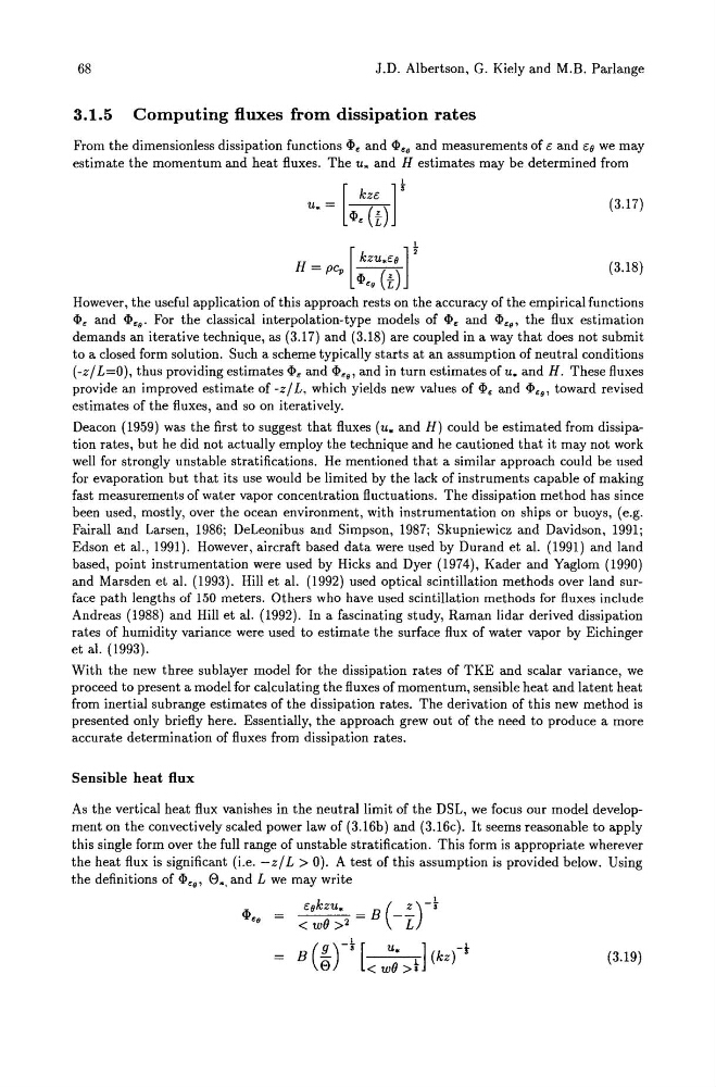
From the dimensionless dissipation functions ~. and ~ •• and measurements of £ and £0 we may
estimate the momentum and heat fluxes. The u. and H estimates may be determined from
[
kz£ ]!u. = ~. (t)
(3.17)
H = pCp [::u(;) r
(3.18)
However, the useful application of this approach rests on the accuracy of the empirical functions
~. and ~ ••. For the classical interpolation-type models of ~. and ~ •• , the flux estimation
demands an iterative technique, as (3.17) and (3.18) are coupled in a way that does not submit
to a closed form solution. Such a scheme typically starts at an assumption of neutral conditions
(-z/ L=O), thus providing estimates~. and ~ •• , and in turn estimates of u. and H. These fluxes
provide an improved estimate of -z/ L, which yields new values of ~. and ~ •• , toward revised
estimates of the fluxes, and so on iteratively.
Deacon (1959) was the first to suggest that fluxes (u. and H) could be estimated from dissipation rates, but he did not actually employ the technique and he cautioned that it may not work
well for strongly unstable stratifications. He mentioned that a similar approach could be used
for evaporation but that its use would be limited by the lack of instruments capable of making
fast measurements of water vapor concentration fluctuations. The dissipation method has since
been used, mostly, over the ocean environment, with instrumentation on ships or buoys, (e.g.
Fairall and Larsen, 1986; DeLeonibus and Simpson, 1987; Skupniewicz and Davidson, 1991;
Edson et al., 1991). However, aircraft based data were used by Durand et al. (1991) and land
based, point instrumentation were used by Hicks and Dyer (1974), Kader and Yaglom (1990)
and Marsden et al. (1993). Hill et al. (1992) used optical scintillation methods over land surface path lengths of 150 meters. Others who have used scintillation methods for fluxes include
Andreas (1988) and Hill et al. (1992). In a fascinating study, Raman lidar derived dissipation
rates of humidity variance were used to estimate the surface flux of water vapor by Eichinger
et al. (1993).
With the new three sublayer model for the dissipation rates of TKE and scalar variance, we
proceed to present a model for calculating the fluxes of momentum, sensible heat and latent heat
from inertial subrange estimates of the dissipation rates. The derivation of this new method is
presented only briefly here. Essentially, the approach grew out of the need to produce a more
accurate determination of fluxes from dissipation rates.
Sensible heat flux
As the vertical heat flux vanishes in the neutral limit of the DSL, we focus our model development on the convectively scaled power law of (3.16b) and (3.16c). It seems reasonable to apply
this single form over the full range of unstable stratification. This form is appropriate wherever
the heat flux is significant (i.e. -z/ L > 0). A test of this assumption is provided below. Using
the definitions of ~ •• , e., and L we may write
~ •• =
1
£okzu. =B(-!")-'
< wO >2
L
B (!!...)-!- [ u. 1] (kzft
e
< wO >i
(3.19)
J.D. Albertson, G. Kiely and M.B. Parlange
3.1.5 Computing fluxes from dissipation rates
From the dimensionless dissipation functions ~. and ~ •• and measurements of £ and £0 we may
estimate the momentum and heat fluxes. The u. and H estimates may be determined from
[
kz£ ]!u. = ~. (t)
(3.17)
H = pCp [::u(;) r
(3.18)
However, the useful application of this approach rests on the accuracy of the empirical functions
~. and ~ ••. For the classical interpolation-type models of ~. and ~ •• , the flux estimation
demands an iterative technique, as (3.17) and (3.18) are coupled in a way that does not submit
to a closed form solution. Such a scheme typically starts at an assumption of neutral conditions
(-z/ L=O), thus providing estimates~. and ~ •• , and in turn estimates of u. and H. These fluxes
provide an improved estimate of -z/ L, which yields new values of ~. and ~ •• , toward revised
estimates of the fluxes, and so on iteratively.
Deacon (1959) was the first to suggest that fluxes (u. and H) could be estimated from dissipation rates, but he did not actually employ the technique and he cautioned that it may not work
well for strongly unstable stratifications. He mentioned that a similar approach could be used
for evaporation but that its use would be limited by the lack of instruments capable of making
fast measurements of water vapor concentration fluctuations. The dissipation method has since
been used, mostly, over the ocean environment, with instrumentation on ships or buoys, (e.g.
Fairall and Larsen, 1986; DeLeonibus and Simpson, 1987; Skupniewicz and Davidson, 1991;
Edson et al., 1991). However, aircraft based data were used by Durand et al. (1991) and land
based, point instrumentation were used by Hicks and Dyer (1974), Kader and Yaglom (1990)
and Marsden et al. (1993). Hill et al. (1992) used optical scintillation methods over land surface path lengths of 150 meters. Others who have used scintillation methods for fluxes include
Andreas (1988) and Hill et al. (1992). In a fascinating study, Raman lidar derived dissipation
rates of humidity variance were used to estimate the surface flux of water vapor by Eichinger
et al. (1993).
With the new three sublayer model for the dissipation rates of TKE and scalar variance, we
proceed to present a model for calculating the fluxes of momentum, sensible heat and latent heat
from inertial subrange estimates of the dissipation rates. The derivation of this new method is
presented only briefly here. Essentially, the approach grew out of the need to produce a more
accurate determination of fluxes from dissipation rates.
Sensible heat flux
As the vertical heat flux vanishes in the neutral limit of the DSL, we focus our model development on the convectively scaled power law of (3.16b) and (3.16c). It seems reasonable to apply
this single form over the full range of unstable stratification. This form is appropriate wherever
the heat flux is significant (i.e. -z/ L > 0). A test of this assumption is provided below. Using
the definitions of ~ •• , e., and L we may write
~ •• =
1
£okzu. =B(-!")-'
< wO >2
L
B (!!...)-!- [ u. 1] (kzft
e
< wO >i
(3.19)