

Monthly and seasonal evapotranspiration “maps” are derived from a series of
ET r F images by interpolating ET r F on a pixel-by-pixel basis between processed
images and multiplying, on a daily basis, by the ET r for each day. The interpolation
of ET r F between image dates is not unlike the construction of a seasonal K c curve
(Allen et al. 1998), where interpolation is done between discrete values for K c .
The METRIC approach assumes that the ET for the entire area of interest
changes in proportion to change in ET r at the weather station. This is a generally
valid assumption and is similar to the assumptions used in the conventional
application of K c  ET r . This approach is effective in estimating ET for both
clear and cloudy days between the clear-sky satellite image dates. Tasumi et al.
(2005) showed that the ET r F was consistent between clear and cloudy days using
lysimeter measurements at Kimberly, Idaho. ET r is computed at a specific weather
station location and therefore may not represent the actual condition at each pixel.
However, because ET r is used only as an index of the relative change in weather,
specific information at each pixel is retained through the ET r F.
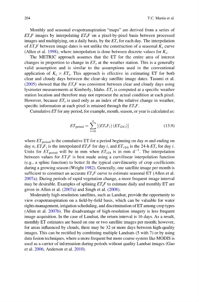
Cumulative ET for any period, for example, month, season, or year is calculated as:
ET period ¼
X n
i¼m
ET r F i
ð
Þ ET r24 i
ð
Þ
½
(13.9)
where ET period is the cumulative ET for a period beginning on day m and ending on
day n, ET r F i is the interpolated ET r F for day i, and ET r24i is the 24-h ET r for day i.
Units for ET period will be in mm when ET r24 is in mm d
À1 . The interpolation
between values for ET r F is best made using a curvilinear interpolation function
(e.g., a spline function) to better fit the typical curvilinearity of crop coefficients
during a growing season (Wright 1982). Generally, one satellite image per month is
sufficient to construct an accurate ET r F curve to estimate seasonal ET (Allen et al.
2007a). During periods of rapid vegetation change, a more frequent image interval
may be desirable. Examples of splining ET r F to estimate daily and monthly ET are
given in Allen et al. (2007a) and Singh et al. (2008).
Moderately high-resolution satellites, such as Landsat, provide the opportunity to
view evapotranspiration on a field-by-field basis, which can be valuable for water
rights management, irrigation scheduling, and discrimination of ET among crop types
(Allen et al. 2007b). The disadvantage of high-resolution imagery is less frequent
image acquisition. In the case of Landsat, the return interval is 16 days. As a result,
monthly ET estimates are based on one or two satellite images per month; however,
for areas influenced by clouds, there may be 32 or more days between high-quality
images. This can be rectified by combining multiple Landsats (5 with 7) or by using
data fusion techniques, where a more frequent but more coarse system like MODIS is
used as a carrier of information during periods without quality Landsat images (Gao
et al. 2006; Anderson et al. 2010).
204
T.C. Martin et al.
ET r F images by interpolating ET r F on a pixel-by-pixel basis between processed
images and multiplying, on a daily basis, by the ET r for each day. The interpolation
of ET r F between image dates is not unlike the construction of a seasonal K c curve
(Allen et al. 1998), where interpolation is done between discrete values for K c .
The METRIC approach assumes that the ET for the entire area of interest
changes in proportion to change in ET r at the weather station. This is a generally
valid assumption and is similar to the assumptions used in the conventional
application of K c  ET r . This approach is effective in estimating ET for both
clear and cloudy days between the clear-sky satellite image dates. Tasumi et al.
(2005) showed that the ET r F was consistent between clear and cloudy days using
lysimeter measurements at Kimberly, Idaho. ET r is computed at a specific weather
station location and therefore may not represent the actual condition at each pixel.
However, because ET r is used only as an index of the relative change in weather,
specific information at each pixel is retained through the ET r F.
Cumulative ET for any period, for example, month, season, or year is calculated as:
ET period ¼
X n
i¼m
ET r F i
ð
Þ ET r24 i
ð
Þ
½
(13.9)
where ET period is the cumulative ET for a period beginning on day m and ending on
day n, ET r F i is the interpolated ET r F for day i, and ET r24i is the 24-h ET r for day i.
Units for ET period will be in mm when ET r24 is in mm d
À1 . The interpolation
between values for ET r F is best made using a curvilinear interpolation function
(e.g., a spline function) to better fit the typical curvilinearity of crop coefficients
during a growing season (Wright 1982). Generally, one satellite image per month is
sufficient to construct an accurate ET r F curve to estimate seasonal ET (Allen et al.
2007a). During periods of rapid vegetation change, a more frequent image interval
may be desirable. Examples of splining ET r F to estimate daily and monthly ET are
given in Allen et al. (2007a) and Singh et al. (2008).
Moderately high-resolution satellites, such as Landsat, provide the opportunity to
view evapotranspiration on a field-by-field basis, which can be valuable for water
rights management, irrigation scheduling, and discrimination of ET among crop types
(Allen et al. 2007b). The disadvantage of high-resolution imagery is less frequent
image acquisition. In the case of Landsat, the return interval is 16 days. As a result,
monthly ET estimates are based on one or two satellite images per month; however,
for areas influenced by clouds, there may be 32 or more days between high-quality
images. This can be rectified by combining multiple Landsats (5 with 7) or by using
data fusion techniques, where a more frequent but more coarse system like MODIS is
used as a carrier of information during periods without quality Landsat images (Gao
et al. 2006; Anderson et al. 2010).
204
T.C. Martin et al.