

Janssen and van Ittersum 2007). The LP model for farm analysis is explained in
detail by Ten Berge et al. (2000) and the use of LP is very sophisticated in modeling
without high additional costs in terms of programming development, and therefore
could be used smoothly in producing the results from the models (Leleu 2006).
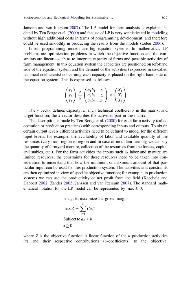
Linear programming models are big equation systems. In mathematics, LP
problems are optimization problems in which the objective function and the constraints are linear—such as to integrate capacity of farms and possible activities of
farm management. In this equation system the capacities are positioned on left-hand
side of the equation system and the demand of the activities (expressed in so-called
technical coefficients) concerning each capacity is placed on the right-hand side of
the equation system. This is expressed as follows:
y 1
y 2
y 3
0
@
1
A !
a 1 b 1 . . .z 1
a 2 b 2 . . .z 2
a 3 b 3 . . .z 3
0
@
1
A Â
X 1
X 2
X 3
0
@
1
A
The y vector defines capacity, a, b…z technical coefficients in the matrix, and
target function; the x vector describes the activities part in the matrix.
The description is made by Ten Berge et al. (2000) for each farm activity (called
operation or production practices) with corresponding inputs and outputs. To obtain
certain output levels different activities need to be defined to model for the different
input levels, for example, the availability of labor and available quantity of the
resources (vary from region to region and in case of mountain farming we can say
the quantity of farmyard manure, collection of the resources from the forests, capital
and stables, etc.). For the farm activities the inputs such as labor and manure are
limited resources; the constraints for these resources need to be taken into consideration to understand that how the minimum or maximum amount of that particular input can be used for this production system. The activities and constraints
are then optimized in view of specific objective function; for example, in production
systems we can use the productivity or net profit from the field (Kaechele and
Dabbert 2002; Zander 2003; Janssen and van Ittersum 2007). The standard mathematical notation for the LP model can be represented by max ≥ 0.
à e.g. to maximize the gross margin
max Z ¼
X m
i¼1
C i x
À
i
Subject to ax b
x ! 0
where Z is the objective function: a linear function of the n production activities
(x) and their respective contributions (c–coefficients) to the objective.
Socioeconomic and Ecological Modeling for Sustainable …
617