

Thermal Land-surface Variables From METEOSAT-IR Data
285
45
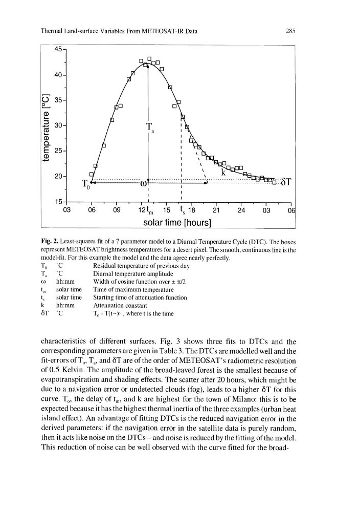
Fig. 2. Least-squares fit of a 7 parameter model to a Diurnal Temperature Cycle (DTC). The boxes
represent METEOSAT brightness temperatures for a desert pixel. The smooth, continuous line is the
model-fit. For this example the model and the data agree nearly perfectly.
To'C
Residual temperature of previous day
Ta
'C
Diurnal temperature amplitude
w
hh:mm
Width of cosine function over ± 1t/2
~
solar time
ts
solar time
k
hh:mm
oT 'C
Time of maximum temperature
Starting time of attenuation function
Attenuation constant
To - T(t~~ , where t is the time
characteristics of different surfaces. Fig. 3 shows three fits to DTCs and the
corresponding parameters are given in Table 3. The DTCs are modelled well and the
fit-errors of To, T a , and aT are of the order of METE OS AT's radiometric resolution
of 0.5 Kelvin. The amplitude of the broad-leaved forest is the smallest because of
evapotranspiration and shading effects. The scatter after 20 hours, which might be
due to a navigation error or undetected clouds (fog), leads to a higher aT for this
curve. To, the delay of tm, and k are highest for the town of Milano: this is to be
expected because it has the highest thermal inertia of the three examples (urban heat
island effect). An advantage of fitting DTCs is the reduced navigation error in the
derived parameters: if the navigation error in the satellite data is purely random,
then it acts like noise on the DTCs - and noise is reduced by the fitting ofthe model.
This reduction of noise can be well observed with the curve fitted for the broad-
285
45
Fig. 2. Least-squares fit of a 7 parameter model to a Diurnal Temperature Cycle (DTC). The boxes
represent METEOSAT brightness temperatures for a desert pixel. The smooth, continuous line is the
model-fit. For this example the model and the data agree nearly perfectly.
To'C
Residual temperature of previous day
Ta
'C
Diurnal temperature amplitude
w
hh:mm
Width of cosine function over ± 1t/2
~
solar time
ts
solar time
k
hh:mm
oT 'C
Time of maximum temperature
Starting time of attenuation function
Attenuation constant
To - T(t~~ , where t is the time
characteristics of different surfaces. Fig. 3 shows three fits to DTCs and the
corresponding parameters are given in Table 3. The DTCs are modelled well and the
fit-errors of To, T a , and aT are of the order of METE OS AT's radiometric resolution
of 0.5 Kelvin. The amplitude of the broad-leaved forest is the smallest because of
evapotranspiration and shading effects. The scatter after 20 hours, which might be
due to a navigation error or undetected clouds (fog), leads to a higher aT for this
curve. To, the delay of tm, and k are highest for the town of Milano: this is to be
expected because it has the highest thermal inertia of the three examples (urban heat
island effect). An advantage of fitting DTCs is the reduced navigation error in the
derived parameters: if the navigation error in the satellite data is purely random,
then it acts like noise on the DTCs - and noise is reduced by the fitting ofthe model.
This reduction of noise can be well observed with the curve fitted for the broad-