

392
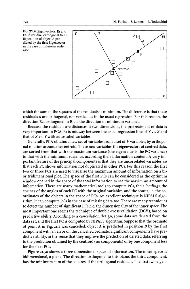
Fig. 21.4. Eigenvectors, El and
E2. d: residual orthogonal to El;
B: position of object A predicted by the first Eigenvector
in the case of unknown ordinate
M. Forina . S. Lanteri . R. Todeschini
which the sum of the squares of the residuals is minimum. The difference is that these
residuals d are orthogonal, not vertical as in the usual regression. For this reason, the
direction E2, orthogonal to E1, is the direction of minimum variance.
Because the residuals are distances it two dimensions, the pretreatment of data is
very important in peA. E1 is midway between the usual regression line of Yvs. X and
that of X vs. Y with auto scaled variables.
Generally, peA obtains a new set of variables from a set of V variables, by orthogonal rotation around the centroid. These new variables, the eigenvectors of centred data,
are sorted from that with the maximum variance (the eigenvalue is the pe variance)
to that with the minimum variance, according their information content. A very important feature of the principal components is that they are uncorrelated variables, so
that each pe shows information not duplicated in other pes. For this reason the first
two or three pes are used to visualise the maximum amount of information on a bior tridimensional plot. The space of the first pes can be considered as the optimum
window opened in the space of the total information to see the maximum amount of
information. There are many mathematical tools to compute pes, their loadings, the
cosines of the angles of each pe with the original variables, and the scores, i.e. the coordinates of the objects in the space of pes. An excellent technique is NIPALS algorithm, it can compute pes in the case of missing data too. There are many techniques
to detect the number of significant pes, i.e. the dimensionality of the inner space. The
most important one seems the technique of double-cross validation (DeV), based on
predictive ability. According to a cancellation design, some data are deleted from the
data set, and the first pe is computed by NIPALS algorithm. Suppose that the ordinate
of point A in Fig. 21.4 was cancelled; object A is predicted in position B by the first
component with an error on the cancelled ordinate. Significant components have predictive ability, in the sense that they improve the prediction of deleted data, referring
to the prediction obtained by the centroid (no components) or by one component less
for the next pes.
Figure 21.5a shows a three dimensional space of information. The inner space is
bidimensional, a plane. The direction orthogonal to this plane, the third component,
has the minimum sum of the squares of the orthogonal residuals. The first two eigen-
Fig. 21.4. Eigenvectors, El and
E2. d: residual orthogonal to El;
B: position of object A predicted by the first Eigenvector
in the case of unknown ordinate
M. Forina . S. Lanteri . R. Todeschini
which the sum of the squares of the residuals is minimum. The difference is that these
residuals d are orthogonal, not vertical as in the usual regression. For this reason, the
direction E2, orthogonal to E1, is the direction of minimum variance.
Because the residuals are distances it two dimensions, the pretreatment of data is
very important in peA. E1 is midway between the usual regression line of Yvs. X and
that of X vs. Y with auto scaled variables.
Generally, peA obtains a new set of variables from a set of V variables, by orthogonal rotation around the centroid. These new variables, the eigenvectors of centred data,
are sorted from that with the maximum variance (the eigenvalue is the pe variance)
to that with the minimum variance, according their information content. A very important feature of the principal components is that they are uncorrelated variables, so
that each pe shows information not duplicated in other pes. For this reason the first
two or three pes are used to visualise the maximum amount of information on a bior tridimensional plot. The space of the first pes can be considered as the optimum
window opened in the space of the total information to see the maximum amount of
information. There are many mathematical tools to compute pes, their loadings, the
cosines of the angles of each pe with the original variables, and the scores, i.e. the coordinates of the objects in the space of pes. An excellent technique is NIPALS algorithm, it can compute pes in the case of missing data too. There are many techniques
to detect the number of significant pes, i.e. the dimensionality of the inner space. The
most important one seems the technique of double-cross validation (DeV), based on
predictive ability. According to a cancellation design, some data are deleted from the
data set, and the first pe is computed by NIPALS algorithm. Suppose that the ordinate
of point A in Fig. 21.4 was cancelled; object A is predicted in position B by the first
component with an error on the cancelled ordinate. Significant components have predictive ability, in the sense that they improve the prediction of deleted data, referring
to the prediction obtained by the centroid (no components) or by one component less
for the next pes.
Figure 21.5a shows a three dimensional space of information. The inner space is
bidimensional, a plane. The direction orthogonal to this plane, the third component,
has the minimum sum of the squares of the orthogonal residuals. The first two eigen-